ไปยังเนื้อหาหลัก

วิธีแสดงรายการอินสแตนซ์ที่ตรงกันทั้งหมดของค่าใน Excel

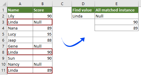
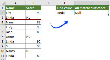
เมื่อภาพหน้าจอด้านซ้ายแสดงขึ้นคุณจะต้องค้นหาและแสดงรายการอินสแตนซ์ที่ตรงกันทั้งหมดของค่า "Linda" ในตาราง จะบรรลุได้อย่างไร? โปรดลองใช้วิธีการในบทความนี้

แสดงรายการอินสแตนซ์ที่ตรงกันทั้งหมดของค่าด้วยสูตรอาร์เรย์
แสดงรายการเฉพาะอินสแตนซ์แรกที่ตรงกันของค่าด้วย Kutools for Excel

บทช่วยสอนเพิ่มเติมสำหรับ VLOOKUP ...


แสดงรายการอินสแตนซ์ที่ตรงกันทั้งหมดของค่าด้วยสูตรอาร์เรย์

ด้วยสูตรอาร์เรย์ต่อไปนี้คุณสามารถแสดงรายการอินสแตนซ์ที่ตรงกันทั้งหมดของค่าในตารางบางตารางใน Excel ได้อย่างง่ายดาย กรุณาดำเนินการดังนี้

1. เลือกเซลล์ว่างเพื่อส่งออกอินสแตนซ์แรกที่ตรงกันป้อนสูตรด้านล่างลงไปจากนั้นกดปุ่ม Ctrl + เปลี่ยน + เข้าสู่ คีย์พร้อมกัน 

=INDEX($B$2:$B$11, SMALL(IF($D$2=$A$2:$A$11, ROW($A$2:$A$11)-ROW($A$2)+1), ROW(1:1)))

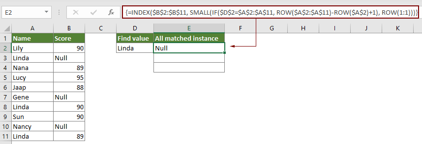
หมายเหตุ: ในสูตร B2: B11 คือช่วงที่อินสแตนซ์ที่ตรงกันค้นหาใน A2: A11 คือช่วงที่มีค่าบางอย่างที่คุณจะแสดงรายการอินสแตนซ์ทั้งหมดตาม และ D2 ประกอบด้วยค่าที่แน่นอน

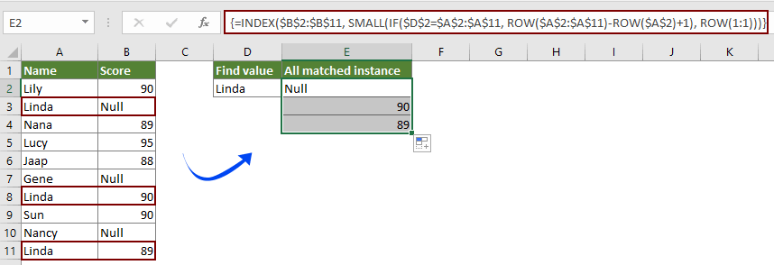
2. เลือกเซลล์ผลลัพธ์จากนั้นลาก Fill Handle ลงเพื่อรับอินสแตนซ์อื่นที่ตรงกัน


แสดงรายการเฉพาะอินสแตนซ์แรกที่ตรงกันของค่าด้วย Kutools for Excel

คุณสามารถค้นหาและแสดงรายการอินสแตนซ์แรกที่ตรงกันของค่าได้อย่างง่ายดายด้วย มองหาค่าในรายการ ฟังก์ชั่น Kutools สำหรับ Excel โดยไม่จำสูตร กรุณาดำเนินการดังนี้

ก่อนที่จะใช้ Kutools สำหรับ Excelโปรด ดาวน์โหลดและติดตั้งในตอนแรก.

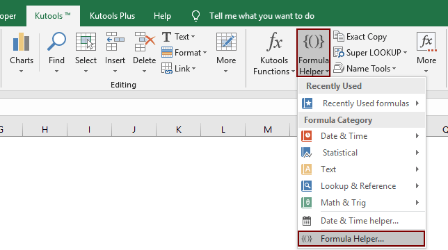
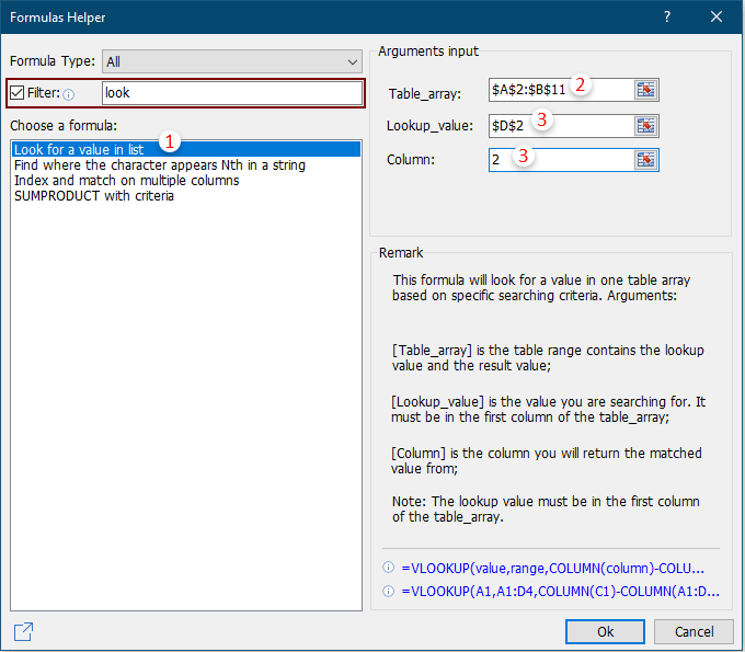
1. เลือกเซลล์ว่างที่คุณจะวางอินสแตนซ์แรกที่ตรงกันจากนั้นคลิก Kutools > ตัวช่วยสูตร > ตัวช่วยสูตร

2 ใน ตัวช่วยสูตร คุณต้อง:

2.1 ค้นหาและเลือก มองหาค่าในรายการ ตัวเลือกใน เลือกสูตร กล่อง;
เคล็ดลับ: คุณสามารถตรวจสอบไฟล์ ตัวกรอง ป้อนคำสำคัญลงในกล่องข้อความเพื่อกรองสูตรที่คุณต้องการอย่างรวดเร็ว
2.2 ใน Table_array เลือกช่วงของตารางซึ่งมีทั้งคอลัมน์ค่าเฉพาะและคอลัมน์อินสแตนซ์ที่ตรงกัน
2.3 ใน ดู_ค่า เลือกเซลล์ที่มีค่าเฉพาะที่คุณจะแสดงรายการอินสแตนซ์แรกตาม;
2.4 ใน คอลัมน์ เลือกคอลัมน์ที่มีอินสแตนซ์ที่ตรงกัน หรือเพียงแค่ใส่หมายเลขคอลัมน์ลงไป
เคล็ดลับ: หมายเลขคอลัมน์จะขึ้นอยู่กับจำนวนคอลัมน์ที่เลือกหากคุณเลือกสี่คอลัมน์และนี่คือคอลัมน์ที่ 3 คุณจะต้องป้อนหมายเลข 3 ลงใน คอลัมน์ กล่อง.
2.5 คลิกที่ไฟล์ OK ปุ่ม 

จากนั้นอินสแตนซ์ที่จับคู่แรกของค่าที่กำหนดจะแสดงตามภาพด้านล่างที่แสดง

  หากคุณต้องการทดลองใช้ยูทิลิตีนี้ฟรี (30 วัน) กรุณาคลิกเพื่อดาวน์โหลดแล้วไปใช้การดำเนินการตามขั้นตอนข้างต้น


บทความที่เกี่ยวข้อง

ค่า Vlookup ในหลายแผ่นงาน
คุณสามารถใช้ฟังก์ชัน vlookup เพื่อส่งคืนค่าที่ตรงกันในตารางของแผ่นงาน อย่างไรก็ตามหากคุณต้องการค่า vlookup ในแผ่นงานหลายแผ่นคุณจะทำอย่างไร? บทความนี้แสดงขั้นตอนโดยละเอียดเพื่อช่วยให้คุณแก้ปัญหาได้อย่างง่ายดาย

Vlookup และส่งคืนค่าที่ตรงกันในหลายคอลัมน์
โดยปกติการใช้ฟังก์ชัน Vlookup สามารถส่งคืนค่าที่ตรงกันจากคอลัมน์เดียวเท่านั้น บางครั้งคุณอาจต้องดึงค่าที่ตรงกันจากหลายคอลัมน์ตามเกณฑ์ นี่คือทางออกสำหรับคุณ

Vlookup เพื่อส่งคืนค่าหลายค่าในเซลล์เดียว
โดยปกติเมื่อใช้ฟังก์ชัน VLOOKUP หากมีหลายค่าที่ตรงกับเกณฑ์คุณจะได้ผลลัพธ์ของค่าแรกเท่านั้น หากคุณต้องการส่งคืนผลลัพธ์ที่ตรงกันทั้งหมดและแสดงผลลัพธ์ทั้งหมดในเซลล์เดียวคุณจะบรรลุได้อย่างไร?

Vlookup และส่งคืนทั้งแถวของค่าที่ตรงกัน
โดยปกติการใช้ฟังก์ชัน vlookup สามารถส่งคืนผลลัพธ์จากคอลัมน์บางคอลัมน์ในแถวเดียวกันเท่านั้น บทความนี้จะแสดงวิธีส่งคืนข้อมูลทั้งแถวตามเกณฑ์เฉพาะ

ย้อนกลับ Vlookup หรือในลำดับย้อนกลับ
โดยทั่วไปฟังก์ชัน VLOOKUP จะค้นหาค่าจากซ้ายไปขวาในตารางอาร์เรย์และต้องการให้ค่าการค้นหาต้องอยู่ทางด้านซ้ายของค่าเป้าหมาย แต่บางครั้งคุณอาจทราบค่าเป้าหมายและต้องการหาค่าการค้นหาในทางกลับกัน ดังนั้นคุณต้อง vlookup ย้อนกลับใน Excel มีหลายวิธีในบทความนี้เพื่อจัดการกับปัญหานี้อย่างง่ายดาย!

บทช่วยสอนเพิ่มเติมสำหรับ VLOOKUP ...

สุดยอดเครื่องมือเพิ่มผลผลิตในสำนักงาน

🤖 Kutools AI ผู้ช่วย: ปฏิวัติการวิเคราะห์ข้อมูลโดยยึดตาม: การดำเนินการที่ชาญฉลาด   |  สร้างรหัส  |  สร้างสูตรที่กำหนดเอง  |  วิเคราะห์ข้อมูลและสร้างแผนภูมิ  |  เรียกใช้ฟังก์ชัน Kutools...
คุณสมบัติยอดนิยม: ค้นหา เน้น หรือระบุรายการที่ซ้ำกัน   |  ลบแถวว่าง   |  รวมคอลัมน์หรือเซลล์โดยไม่สูญเสียข้อมูล   |   รอบโดยไม่มีสูตร ...
การค้นหาขั้นสูง: VLookup หลายเกณฑ์    VLookup หลายค่า  |   VLookup ข้ามหลายแผ่น   |   การค้นหาที่ไม่ชัดเจน ....
รายการแบบเลื่อนลงขั้นสูง: สร้างรายการแบบหล่นลงอย่างรวดเร็ว   |  รายการแบบหล่นลงขึ้นอยู่กับ   |  เลือกหลายรายการแบบหล่นลง ....
ผู้จัดการคอลัมน์: เพิ่มจำนวนคอลัมน์เฉพาะ  |  ย้ายคอลัมน์  |  สลับสถานะการมองเห็นของคอลัมน์ที่ซ่อนอยู่  |  เปรียบเทียบช่วงและคอลัมน์ ...
คุณสมบัติเด่น: กริดโฟกัส   |  มุมมองการออกแบบ   |   บาร์สูตรใหญ่    สมุดงานและตัวจัดการชีต   |  ห้องสมุดทรัพยากร (ข้อความอัตโนมัติ)   |  เลือกวันที่   |  รวมแผ่นงาน   |  เข้ารหัส/ถอดรหัสเซลล์    ส่งอีเมลตามรายการ   |  ซุปเปอร์ฟิลเตอร์   |   ตัวกรองพิเศษ (กรองตัวหนา/ตัวเอียง/ขีดทับ...) ...
ชุดเครื่องมือ 15 อันดับแรก12 ข้อความ เครื่องมือ (เพิ่มข้อความ, ลบอักขระ, ... )   |   50 + แผนภูมิ ประเภท (แผนภูมิ Gantt, ... )   |   40+ ใช้งานได้จริง สูตร (คำนวณอายุตามวันเกิด, ... )   |   19 การแทรก เครื่องมือ (ใส่ QR Code, แทรกรูปภาพจากเส้นทาง, ... )   |   12 การแปลง เครื่องมือ (ตัวเลขเป็นคำ, การแปลงสกุลเงิน, ... )   |   7 ผสานและแยก เครื่องมือ (แถวรวมขั้นสูง, แยกเซลล์, ... )   |   ... และอื่น ๆ

เพิ่มพูนทักษะ Excel ของคุณด้วย Kutools สำหรับ Excel และสัมผัสประสิทธิภาพอย่างที่ไม่เคยมีมาก่อน Kutools สำหรับ Excel เสนอคุณสมบัติขั้นสูงมากกว่า 300 รายการเพื่อเพิ่มประสิทธิภาพและประหยัดเวลา  คลิกที่นี่เพื่อรับคุณสมบัติที่คุณต้องการมากที่สุด...

รายละเอียด


แท็บ Office นำอินเทอร์เฟซแบบแท็บมาที่ Office และทำให้งานของคุณง่ายขึ้นมาก

  • เปิดใช้งานการแก้ไขและอ่านแบบแท็บใน Word, Excel, PowerPoint, ผู้จัดพิมพ์, Access, Visio และโครงการ
  • เปิดและสร้างเอกสารหลายรายการในแท็บใหม่ของหน้าต่างเดียวกันแทนที่จะเป็นในหน้าต่างใหม่
  • เพิ่มประสิทธิภาพการทำงานของคุณ 50% และลดการคลิกเมาส์หลายร้อยครั้งให้คุณทุกวัน!
Comments (15)
Rated 5 out of 5 · 1 ratings
This comment was minimized by the moderator on the site
Is there a way to make it totla up the values it find and just put it in the first box?
This comment was minimized by the moderator on the site
Hi Bramdon,

To total up all matched values, the following formula can help. Or you can take a look at this tutorial: vlookup and sum matches in rows or columns in Excel
=SUMPRODUCT((A2:A7=A10)*B2:F7)
https://www.extendoffice.com/images/stories/doc-excel/doc-vlookup-and-sum/doc-vlookup-sum-sumif4.png
This comment was minimized by the moderator on the site
Is there a way to stop this formula returning duplicate values

Thanks
Steven
This comment was minimized by the moderator on the site
Hi Steven Waddleton,
The following two formulas can do you a favor.
Array formula in E2:
=INDEX($B$2:$B$11,MATCH(0,COUNTIF($E$1:E1,$B$2:$B$11)+($A$2:$A$11<>$D$2),0)) + Ctrl + Shift + Enter
Formula in E2:
=LOOKUP(2, 1/((COUNTIF($F$1:F1,$B$2:$B$11)=0)*($D$2=$A$2:$A$11)), $B$2:$B$11)
In the formulas, E1 is the cell above the result cell.
https://www.extendoffice.com/images/stories/comments/comment-picture-zxm/instance-no-duplicates.png
This comment was minimized by the moderator on the site
WOW! Worked perfectly, thanks a ton! Awesome formula.
Rated 5 out of 5
This comment was minimized by the moderator on the site
Nice formula. In testing it I get #NUMBER! when I clear cells A9:B11. How to change the formula to prevent getting this error? I wonder, because I want to use this formula for a list of events on a certain date and on date 1 there are 40 events, on day 2 it are 10 events etc. I could create an indexed list for perhaps 100 rows, but it looks very strange when for date 2 the first 10 rows show events and the other 90 rows show #NUMBER!. It would be okay for me if it gave "-" as a result instead of #NUMBER!
This comment was minimized by the moderator on the site
Fantastic. Thank you so much. Very helpful for my work.
This comment was minimized by the moderator on the site
Amazing. The formula worked for me exactly the way I was looking for. Hats off. Thanks a ton
This comment was minimized by the moderator on the site
Question, I have a sheet laid out opposite of this where "Linda" would be the column header I would like to flag on and the value "90" or 89" I would like to return. Would I change the row function to a column function?
This comment was minimized by the moderator on the site
How would I use this formula but instead of filling down I could fill across but the formula would continue moving down as I fill across (ie. the formula changes from ROW(1:1) to ROW(2:2)
This comment was minimized by the moderator on the site
Hi Luke,The below array formula can do you a favor. Note: After entering the formula, please press the Ctrl + Shift + Enter key to apply it. And then drag its Fill Handle right across the cells you need. =INDEX($B$2:$B$11, SMALL(IF($D$2=$A$2:$A$11, ROW($A$2:$A$11)-ROW($A$2)+1), COLUMN(A1)))
This comment was minimized by the moderator on the site
A very useful and educational formula. I am matching against a set numeric value and it works a treat. How can I use >= rather than just = (i.e. IF($D$2>=$A$2:$A$11) to perform the match so it is looking for values greater than a set value (in $D$2). I assume as it doesn't work as one of the functions in the formula is matching against specific text rather than working with numbers?
This comment was minimized by the moderator on the site
This was super useful, thanks! I'm trying to take this one step further and be able to return all match instances of a certain value while having to search through more than a single-column array. To work through this using your example, I added a second column of test scores and modified your formula to look up a given test score and return the names that match that score. I got this to work with INDEX(SMALL()) and can pull all of the names from both test columns. I've also managed to return only names with that score on Test 2 using INDEX(MATCH(INDEX(MATCH))), however this can only find the first instance in the array. What I'm really trying to do is a combination of these: return all of the names with the given array, while narrowing the search to a specific column within the array. Do you have any tips for this?
This comment was minimized by the moderator on the site
Good day,
Would you please provide a screenshot of your spreadsheet showing what you are exactly trying to do? Thank you for your comment.
There are no comments posted here yet
Load More
Please leave your comments in English
Posting as Guest
×
Rate this post:
0   Characters
Suggested Locations