ไปยังเนื้อหาหลัก

วิธี vlookup และรวมการจับคู่ในแถวหรือคอลัมน์ใน Excel

การใช้ vlookup และฟังก์ชัน sum ช่วยให้คุณค้นหาเกณฑ์ที่ระบุได้อย่างรวดเร็วและรวมค่าที่เกี่ยวข้องในเวลาเดียวกัน ในบทความนี้เราจะแสดงวิธีการสองวิธีในการ vlookup และรวมค่าแรกหรือทั้งหมดที่ตรงกันในแถวหรือคอลัมน์ใน Excel

Vlookup และผลรวมที่ตรงกันในแถวหรือหลายแถวด้วยสูตร
Vlookup และผลรวมที่ตรงกันในคอลัมน์ที่มีสูตร
vlookup และรวมการจับคู่ในแถวหรือคอลัมน์ได้อย่างง่ายดายด้วยเครื่องมือที่น่าทึ่ง

บทช่วยสอนเพิ่มเติมสำหรับ VLOOKUP ...


Vlookup และผลรวมที่ตรงกันในแถวหรือหลายแถวด้วยสูตร

สูตรในส่วนนี้สามารถช่วยในการรวมค่าแรกหรือค่าที่ตรงกันทั้งหมดในแถวหรือหลายแถวตามเกณฑ์เฉพาะใน Excel กรุณาดำเนินการดังนี้

Vlookup และรวมค่าที่ตรงกันแรกในแถว

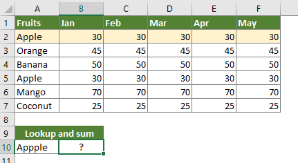
สมมติว่าคุณมีตารางผลไม้ตามภาพด้านล่างที่แสดงและคุณต้องค้นหา Apple เครื่องแรกในตารางจากนั้นรวมค่าที่เกี่ยวข้องทั้งหมดในแถวเดียวกัน เพื่อให้บรรลุสิ่งนี้โปรดทำดังนี้

1. เลือกเซลล์ว่างเพื่อแสดงผลลัพธ์ที่นี่ฉันเลือกเซลล์ B10 คัดลอกสูตรด้านล่างลงไปแล้วกด Ctrl + เปลี่ยน + เข้าสู่ กุญแจสำคัญในการรับผลลัพธ์

=SUM(VLOOKUP(A10, $A$2:$F$7, {2,3,4,5,6}, FALSE))

หมายเหตุ:

  • A10 คือเซลล์ที่มีค่าที่คุณกำลังมองหา
  • $ ก $ 2: $ F $ 7 คือช่วงตารางข้อมูล (ไม่มีส่วนหัว) ซึ่งรวมค่าการค้นหาและค่าที่ตรงกัน
  • จำนวน 2,3,4,5,6 {} แสดงว่าคอลัมน์ค่าผลลัพธ์เริ่มต้นด้วยคอลัมน์ที่สองและลงท้ายด้วยคอลัมน์ที่หกของตาราง หากจำนวนคอลัมน์ผลลัพธ์มากกว่า 6 โปรดเปลี่ยน {2,3,4,5,6} เป็น {2,3,4,5,6,7,8,9 ….}
Vlookup และรวมค่าที่ตรงกันทั้งหมดในหลายแถว

สูตรข้างต้นสามารถรวมค่าในแถวสำหรับค่าแรกที่ตรงกันเท่านั้น หากคุณต้องการส่งคืนผลรวมของการจับคู่ทั้งหมดในหลายแถวโปรดทำดังนี้

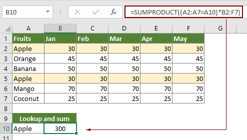
1. เลือกเซลล์ว่าง (ในกรณีนี้ฉันเลือกเซลล์ B10) คัดลอกสูตรด้านล่างลงไปแล้วกดปุ่ม เข้าสู่ กุญแจสำคัญในการรับผลลัพธ์

=SUMPRODUCT((A2:A7=A10)*B2:F7)

vlookup และรวมการจับคู่ในแถวหรือคอลัมน์ใน Excel ได้อย่างง่ายดาย:

พื้นที่ ค้นหาและผลรวม ประโยชน์ของ Kutools สำหรับ Excel สามารถช่วยคุณ vlookup ได้อย่างรวดเร็วและรวมการจับคู่ในแถวหรือคอลัมน์ใน Excel ดังตัวอย่างด้านล่างที่แสดง
ดาวน์โหลดฟีเจอร์เต็มฟรี 30 วันของ Kutools for Excel ตอนนี้!


Vlookup และรวมค่าที่ตรงกันในคอลัมน์ที่มีสูตร

ส่วนนี้แสดงสูตรเพื่อส่งกลับผลรวมของคอลัมน์ใน Excel ตามเกณฑ์ที่ระบุ ตามภาพหน้าจอด้านล่างคุณกำลังมองหาชื่อคอลัมน์ "Jan" ในตารางผลไม้จากนั้นรวมค่าคอลัมน์ทั้งหมด กรุณาดำเนินการดังนี้

1. เลือกเซลล์ว่างคัดลอกสูตรด้านล่างลงไปแล้วกดปุ่ม เข้าสู่ กุญแจสำคัญในการรับผลลัพธ์

=SUM(INDEX(B2:F7,0,MATCH(A10,B1:F1,0)))


vlookup และรวมการจับคู่ในแถวหรือคอลัมน์ได้อย่างง่ายดายด้วยเครื่องมือที่น่าทึ่ง

หากคุณไม่ถนัดในการใช้สูตรขอแนะนำให้คุณใช้ Vlookup และ Sum คุณลักษณะของ Kutools สำหรับ Excel. ด้วยคุณสมบัตินี้คุณสามารถ vlookup และรวมการจับคู่ในแถวหรือคอลัมน์ได้อย่างง่ายดายด้วยการคลิกเพียงครั้งเดียว

ก่อนที่จะใช้ Kutools สำหรับ Excelโปรด ดาวน์โหลดและติดตั้งในตอนแรก.

Vlookup และรวมค่าแรกหรือค่าที่ตรงกันทั้งหมดในแถวหรือหลายแถว

1 คลิก Kutools > สุดยอดการค้นหา > ค้นหาและผลรวม เพื่อเปิดใช้งานคุณสมบัติ ดูภาพหน้าจอ:

2 ใน ค้นหาและผลรวม โปรดกำหนดค่าดังต่อไปนี้

  • 2.1) ใน ค้นหาและประเภทผลรวม เลือก ค้นหาและรวมค่าที่ตรงกันในแถว ตัวเลือก;
  • 2.2) ใน ค้นหาค่า กล่องเลือกเซลล์ที่มีค่าที่คุณต้องการ
  • 2.3) ใน ช่วงเอาท์พุท กล่องเลือกเซลล์เพื่อส่งออกผลลัพธ์
  • 2.4) ใน ช่วงตารางข้อมูล เลือกช่วงของตารางที่ไม่มีส่วนหัวของคอลัมน์
  • 2.5) ใน Options หากคุณต้องการรวมค่าสำหรับค่าแรกที่ตรงกันเท่านั้นให้เลือก ส่งคืนผลรวมของค่าแรกที่ตรงกัน ตัวเลือก หากคุณต้องการรวมค่าสำหรับการจับคู่ทั้งหมดให้เลือก ส่งคืนผลรวมของค่าที่ตรงกันทั้งหมด ตัวเลือก;
  • 2.6) คลิกปุ่ม OK เพื่อรับผลลัพธ์ทันที ดูภาพหน้าจอ:

หมายเหตุ: หากคุณต้องการ vlookup และรวมค่าแรกหรือค่าที่ตรงกันทั้งหมดในคอลัมน์หรือหลายคอลัมน์โปรดตรวจสอบไฟล์ ค้นหาและรวมค่าที่ตรงกันในคอลัมน์ ในกล่องโต้ตอบแล้วกำหนดค่าตามภาพหน้าจอด้านล่างที่แสดง

สำหรับรายละเอียดเพิ่มเติมของคุณสมบัตินี้ โปรดคลิกที่นี่.

  หากคุณต้องการทดลองใช้ยูทิลิตีนี้ฟรี (30 วัน) กรุณาคลิกเพื่อดาวน์โหลดแล้วไปใช้การดำเนินการตามขั้นตอนข้างต้น


บทความที่เกี่ยวข้อง

ค่า Vlookup ในหลายแผ่นงาน
คุณสามารถใช้ฟังก์ชัน vlookup เพื่อส่งคืนค่าที่ตรงกันในตารางของแผ่นงาน อย่างไรก็ตามหากคุณต้องการค่า vlookup ในแผ่นงานหลายแผ่นคุณจะทำอย่างไร? บทความนี้แสดงขั้นตอนโดยละเอียดเพื่อช่วยให้คุณแก้ปัญหาได้อย่างง่ายดาย

Vlookup และส่งคืนค่าที่ตรงกันในหลายคอลัมน์
โดยปกติการใช้ฟังก์ชัน Vlookup สามารถส่งคืนค่าที่ตรงกันจากคอลัมน์เดียวเท่านั้น บางครั้งคุณอาจต้องดึงค่าที่ตรงกันจากหลายคอลัมน์ตามเกณฑ์ นี่คือทางออกสำหรับคุณ

Vlookup เพื่อส่งคืนค่าหลายค่าในเซลล์เดียว
โดยปกติเมื่อใช้ฟังก์ชัน VLOOKUP หากมีหลายค่าที่ตรงกับเกณฑ์คุณจะได้ผลลัพธ์ของค่าแรกเท่านั้น หากคุณต้องการส่งคืนผลลัพธ์ที่ตรงกันทั้งหมดและแสดงผลลัพธ์ทั้งหมดในเซลล์เดียวคุณจะบรรลุได้อย่างไร?

Vlookup และส่งคืนทั้งแถวของค่าที่ตรงกัน
โดยปกติการใช้ฟังก์ชัน vlookup สามารถส่งคืนผลลัพธ์จากคอลัมน์บางคอลัมน์ในแถวเดียวกันเท่านั้น บทความนี้จะแสดงวิธีส่งคืนข้อมูลทั้งแถวตามเกณฑ์เฉพาะ

ย้อนกลับ Vlookup หรือในลำดับย้อนกลับ
โดยทั่วไปฟังก์ชัน VLOOKUP จะค้นหาค่าจากซ้ายไปขวาในตารางอาร์เรย์และต้องการให้ค่าการค้นหาต้องอยู่ทางด้านซ้ายของค่าเป้าหมาย แต่บางครั้งคุณอาจทราบค่าเป้าหมายและต้องการหาค่าการค้นหาในทางกลับกัน ดังนั้นคุณต้อง vlookup ย้อนกลับใน Excel มีหลายวิธีในบทความนี้เพื่อจัดการกับปัญหานี้อย่างง่ายดาย!

บทช่วยสอนเพิ่มเติมสำหรับ VLOOKUP ...

สุดยอดเครื่องมือเพิ่มผลผลิตในสำนักงาน

🤖 Kutools AI ผู้ช่วย: ปฏิวัติการวิเคราะห์ข้อมูลโดยยึดตาม: การดำเนินการที่ชาญฉลาด   |  สร้างรหัส  |  สร้างสูตรที่กำหนดเอง  |  วิเคราะห์ข้อมูลและสร้างแผนภูมิ  |  เรียกใช้ฟังก์ชัน Kutools...
คุณสมบัติยอดนิยม: ค้นหา เน้น หรือระบุรายการที่ซ้ำกัน   |  ลบแถวว่าง   |  รวมคอลัมน์หรือเซลล์โดยไม่สูญเสียข้อมูล   |   รอบโดยไม่มีสูตร ...
การค้นหาขั้นสูง: VLookup หลายเกณฑ์    VLookup หลายค่า  |   VLookup ข้ามหลายแผ่น   |   การค้นหาที่ไม่ชัดเจน ....
รายการแบบเลื่อนลงขั้นสูง: สร้างรายการแบบหล่นลงอย่างรวดเร็ว   |  รายการแบบหล่นลงขึ้นอยู่กับ   |  เลือกหลายรายการแบบหล่นลง ....
ผู้จัดการคอลัมน์: เพิ่มจำนวนคอลัมน์เฉพาะ  |  ย้ายคอลัมน์  |  สลับสถานะการมองเห็นของคอลัมน์ที่ซ่อนอยู่  |  เปรียบเทียบช่วงและคอลัมน์ ...
คุณสมบัติเด่น: กริดโฟกัส   |  มุมมองการออกแบบ   |   บาร์สูตรใหญ่    สมุดงานและตัวจัดการชีต   |  ห้องสมุดทรัพยากร (ข้อความอัตโนมัติ)   |  เลือกวันที่   |  รวมแผ่นงาน   |  เข้ารหัส/ถอดรหัสเซลล์    ส่งอีเมลตามรายการ   |  ซุปเปอร์ฟิลเตอร์   |   ตัวกรองพิเศษ (กรองตัวหนา/ตัวเอียง/ขีดทับ...) ...
ชุดเครื่องมือ 15 อันดับแรก12 ข้อความ เครื่องมือ (เพิ่มข้อความ, ลบอักขระ, ... )   |   50 + แผนภูมิ ประเภท (แผนภูมิ Gantt, ... )   |   40+ ใช้งานได้จริง สูตร (คำนวณอายุตามวันเกิด, ... )   |   19 การแทรก เครื่องมือ (ใส่ QR Code, แทรกรูปภาพจากเส้นทาง, ... )   |   12 การแปลง เครื่องมือ (ตัวเลขเป็นคำ, การแปลงสกุลเงิน, ... )   |   7 ผสานและแยก เครื่องมือ (แถวรวมขั้นสูง, แยกเซลล์, ... )   |   ... และอื่น ๆ

เพิ่มพูนทักษะ Excel ของคุณด้วย Kutools สำหรับ Excel และสัมผัสประสิทธิภาพอย่างที่ไม่เคยมีมาก่อน Kutools สำหรับ Excel เสนอคุณสมบัติขั้นสูงมากกว่า 300 รายการเพื่อเพิ่มประสิทธิภาพและประหยัดเวลา  คลิกที่นี่เพื่อรับคุณสมบัติที่คุณต้องการมากที่สุด...

รายละเอียด


แท็บ Office นำอินเทอร์เฟซแบบแท็บมาที่ Office และทำให้งานของคุณง่ายขึ้นมาก

  • เปิดใช้งานการแก้ไขและอ่านแบบแท็บใน Word, Excel, PowerPoint, ผู้จัดพิมพ์, Access, Visio และโครงการ
  • เปิดและสร้างเอกสารหลายรายการในแท็บใหม่ของหน้าต่างเดียวกันแทนที่จะเป็นในหน้าต่างใหม่
  • เพิ่มประสิทธิภาพการทำงานของคุณ 50% และลดการคลิกเมาส์หลายร้อยครั้งให้คุณทุกวัน!
Comments (26)
No ratings yet. Be the first to rate!
This comment was minimized by the moderator on the site
I need help with a formula. I have 2 sheets to pull data from and calculate the sum of on column with a match to a name.
I.e Name is in sheet 1 D5, the name in sheet 2 is B3 the amounts to calculate which match the name in B3 in sheet 2 is F3 to F32.
I've tried sum index, vlookup, match and so on but keep getting a 0. Can anyone assist with this?
This comment was minimized by the moderator on the site
Hi Marnel Strydom,
I don't know if I understand you correctly: If the name in D5 of Sheet1 matches the name in B3 of Sheet2, then sum numbers in the range F3:F32 of Sheet2.
If so, you can apply the following formula to get it done.
=SUM(INDEX(Sheet2!F3:F32,0,MATCH(Sheet1!D5,Sheet2!B3,0)))
This comment was minimized by the moderator on the site
I have a multi sheet spread sheet keeping track of job hours. I have used VLOOKUP in succession to sum all the hours on multiple sheets and it works great... Until it gets to a sheet that does not contain the lookup value. I have searched all over for my issue, and VLOOKUP may be the incorrect solution. I was wondering if I could rattle anyone's brain to make this work.

I.E. I have 1 excel document with 52 tabs. Each tab is a work week starting from January so WW1 is all the hours FOR sed jobs I did for that week. "joes house 2 hours ; mikes house 3 hours"... WW2, WW3 etc... Until WW52.

This is the function I made to add hours together...

=SUM(VLOOKUP(O30,'WW29'!$A$7:$M$110,{13},FALSE),VLOOKUP(O30,'WW30'!$A$7:$M$110,{13},FALSE),VLOOKUP(O30,'WW31'!$A$7:$M$110,{13},FALSE)) And it works great. But when that job is finished it is not on (for example WW32 tab). Hence I get the #N/A error. so for example, as the previous one works great when I expand the formula to cover all 52 sheets... (EXAMPLE OF NEXT PAGE WIOTHOUT LOOKUP VALUE)

=SUM(VLOOKUP(O30,'WW29'!$A$7:$M$110,{13},FALSE),VLOOKUP(O30,'WW30'!$A$7:$M$110,{13},FALSE),VLOOKUP(O30,'WW31'!$A$7:$M$110,{13},FALSE),VLOOKUP(O30,'WW32'!$A$7:$M$110,{13},FALSE)) I get the #N/A error because the job is not listed on WW32. But I may add hours to that on WW45.

Is there a way to make VLOOKUP skip a sheet that does not have the referenced value and continue summing it till the end? I apologize, this may be as clear as mud but I will clarify anything if need be.

I have also tried IFERROR. You can set IFERROR to return text or even blanks, but does not seem to cover summing. I'm looking for how to SUM multiple sheets when some of the sheets do not contain the lookup value. When using IFERROR function, instead of RETURNING #N/A it just returns "YOU'VE ENTERERED TOO MANY ARGUMENTS FOR THIS FUNCTION"...

=IFERROR(VLOOKUP(O30,'WW29'!$A$7:$M$110,{13},FALSE),VLOOKUP(O30,'WW30'!$A$7:$M$110,{13},FALSE),VLOOKUP(O30,'WW31'!$A$7:$M$110,{13},FALSE),VLOOKUP(O30,'WW32'!$A$7:$M$110,{13},FALSE),"")

And that's just 3 sheets.

Any help would be greatly appreciated.

P.S. I have tried with CTRL+SHIFT+ENTER as well to no avail.
This comment was minimized by the moderator on the site
Hi Joe,
The methods provided in the following article can do you a favor. Please give it a try. Hope I can help.
How To Vlookup Across Multiple Sheets And Sum Results In Excel?
This comment was minimized by the moderator on the site
A B C D E F
1 I want this cells in col B to sum the values in col F7 (today) to say F20. this will reduce as tomorrow it will sum the values from F8:F20 and so on -$19 I
want this cells in column B to sum the values in col F7 (today) to say F10.
this will reduce as tomorrow it will sum the values from F8:F10 and so on

2 Fri 22 Jul 22 -$19
3 Sat 23 Jul 22 -$19
4 Sun 24 Jul 22 -$19
5 Mon 25 Jul 22 -$19
6 Tue 26 Jul 22 -$19
7 Wed 27 Jul 22 -$19 tried with vlookup, needless to say it doesn't work
8 Thu 28 Jul 22 -$19 =L8=(D1-E1)+SUM(vlookup(today(),6,false):F28)
9 Fri 29 Jul 22 -$19
10 Sat 30 Jul 22 -$19
11 Sun 31 Jul 22 -$19
12 Mon 01 Aug 22 -$19
13 Tue 02 Aug 22 -$19
14 Wed 03 Aug 22 -$19
15 Thu 04 Aug 22 -$19
This comment was minimized by the moderator on the site
hi
How can I add multiple vlookups together and sum it up ?


=VLOOKUP(E3,'Waste Process NEW'!N:O,2,FALSE) --------------- for this everything goes fine except that retune valve is only the first one where N column have many values match's lookup values of E3.


using index didn't help and shows #N/A
=SUM(INDEX('Waste Process NEW'!N:N,0,MATCH('Monthly Report'!H5,'Waste Process NEW'!1:1048576,0)))
This comment was minimized by the moderator on the site
Hi tariq,
Would you mind providing a screenshot of your data? Sorry for the inconvenience.
This comment was minimized by the moderator on the site
I just get a #VALUE! when I try to do all matched values, but it works for the first value. Any idea?
This comment was minimized by the moderator on the site
How can I add multiple vlookups together, for example I want to look up from your example Apples + oranges + bananas for January.Is there a way to do this?
This comment was minimized by the moderator on the site
I'm having trouble with a similar formula I feel like I need to use an index but can't figure it out. I'm trying to get the sum but the lookup is based on 2 values. Column D which contains an employee's extension and column I which provides a logout code. The goal is to find the sum of time in column K based on a specific employee (column D) and the logout code (column I).
This comment was minimized by the moderator on the site
Hi Mike,
Do you mind uploading a screenshot of your data?
This comment was minimized by the moderator on the site
Thanks but I was able to get my formula up and running with a sumifs calculation. Sumifs giving the sum of something based on multiple factors. Mine being an employee ID number and a status code.
This comment was minimized by the moderator on the site
what will be the formula to add qty of apple in jan only
This comment was minimized by the moderator on the site
the =SUM(PRODUCT((A2:A7=A11)*B2:I7) is not working with decimal point.
This comment was minimized by the moderator on the site
For me works just fine. Try without separating SUM and Product, it should be =SUMPRODUCT((A2:A7=A11)*B2:I7)
This comment was minimized by the moderator on the site
can one sum things up in a column and not a row?
This comment was minimized by the moderator on the site
Hi Jelly,
This formula =SUM(INDEX(B2:F9,0,MATCH(A12,B1:F1,0))) can help you solve the problem. Please have a try. Hope I can help.
There are no comments posted here yet
Load More
Please leave your comments in English
Posting as Guest
×
Rate this post:
0   Characters
Suggested Locations