ไปยังเนื้อหาหลัก

วิธี จำกัด จำนวนตำแหน่งทศนิยมในสูตรใน Excel

ตัวอย่างเช่นคุณรวมช่วงและรับค่าผลรวมที่มีทศนิยมสี่ตำแหน่งใน Excel คุณอาจนึกถึงการจัดรูปแบบค่าผลรวมนี้เป็นทศนิยมหนึ่งตำแหน่งในกล่องโต้ตอบจัดรูปแบบเซลล์ จริงๆแล้วคุณสามารถ จำกัด จำนวนตำแหน่งทศนิยมในสูตรได้โดยตรง บทความนี้พูดถึงการ จำกัด จำนวนตำแหน่งทศนิยมด้วยคำสั่ง Format Cells และการ จำกัด จำนวนตำแหน่งทศนิยมด้วยสูตร Round ใน Excel

จำกัด จำนวนตำแหน่งทศนิยมด้วยคำสั่ง Format Cell ใน Excel

โดยปกติเราสามารถจัดรูปแบบเซลล์เพื่อ จำกัด จำนวนตำแหน่งทศนิยมใน Excel ได้อย่างง่ายดาย

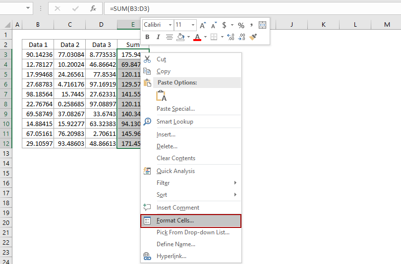
1. เลือกเซลล์ที่คุณต้องการ จำกัด จำนวนตำแหน่งทศนิยม

2. คลิกขวาที่เซลล์ที่เลือกแล้วเลือกไฟล์ จัดรูปแบบเซลล์ จากเมนูคลิกขวา

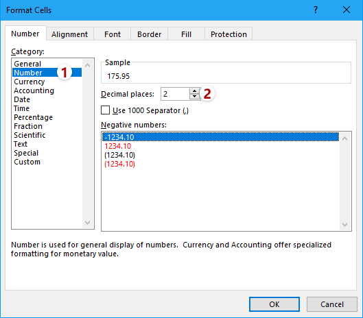
3. ในกล่องโต้ตอบ Format Cells ที่กำลังจะมาให้ไปที่ไฟล์ จำนวน คลิกเพื่อไฮไลต์ จำนวน ใน หมวดหมู่ จากนั้นพิมพ์ตัวเลขในไฟล์ ตำแหน่งทศนิยม กล่อง.
ตัวอย่างเช่นหากคุณต้องการ จำกัด ทศนิยมเพียง 1 ตำแหน่งสำหรับเซลล์ที่เลือกให้พิมพ์ 1 เข้าไปใน ตำแหน่งทศนิยม กล่อง. ดูภาพหน้าจอด้านล่าง:

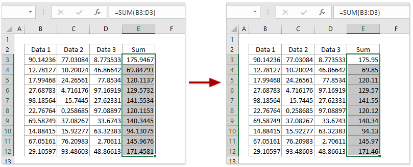
4. คลิก OK ในกล่องโต้ตอบจัดรูปแบบเซลล์ จากนั้นคุณจะเห็นทศนิยมทั้งหมดในเซลล์ที่เลือกเปลี่ยนเป็นทศนิยมหนึ่งตำแหน่ง

หมายเหตุ หลังจากเลือกเซลล์แล้วคุณสามารถคลิกไฟล์ เพิ่มทศนิยม ปุ่ม  or ลดทศนิยม ปุ่ม  โดยตรงในไฟล์ จำนวน กลุ่มใน หน้าแรก เพื่อเปลี่ยนตำแหน่งทศนิยม

จำกัด จำนวนตำแหน่งทศนิยมในหลาย ๆ สูตรใน Excel ได้อย่างง่ายดาย

โดยทั่วไปคุณสามารถใช้ = Round (original_formula, num_digits) เพื่อ จำกัด จำนวนตำแหน่งทศนิยมในสูตรเดียวได้อย่างง่ายดาย อย่างไรก็ตามจะค่อนข้างน่าเบื่อและใช้เวลานานในการปรับเปลี่ยนสูตรทีละสูตรด้วยตนเอง ที่นี่ใช้คุณสมบัติการทำงานของ Kutools for Excel คุณสามารถ จำกัด จำนวนตำแหน่งทศนิยมในหลาย ๆ สูตรได้อย่างง่ายดาย!


Kutools สำหรับ Excel - เพิ่มประสิทธิภาพ Excel ด้วยเครื่องมือที่จำเป็นมากกว่า 300 รายการ เพลิดเพลินกับฟีเจอร์ทดลองใช้ฟรี 30 วันโดยไม่ต้องใช้บัตรเครดิต! Get It Now

จำกัด จำนวนตำแหน่งทศนิยมในสูตรใน Excel

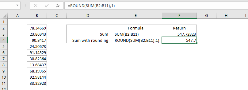
สมมติว่าคุณคำนวณผลรวมของชุดตัวเลขและคุณต้องการ จำกัด จำนวนตำแหน่งทศนิยมสำหรับค่าผลรวมนี้ในสูตรคุณจะทำได้อย่างไรใน Excel คุณควรลองใช้ฟังก์ชัน Round

ไวยากรณ์ของสูตร Round พื้นฐานคือ:

= ROUND (ตัวเลข num_digits)

และถ้าคุณต้องการรวมฟังก์ชัน Round กับสูตรอื่น ๆ ควรเปลี่ยนไวยากรณ์ของสูตรเป็น

= รอบ (original_formula, num_digits)

ในกรณีของเราเราต้องการ จำกัด ทศนิยมหนึ่งตำแหน่งสำหรับค่าผลรวมดังนั้นเราจึงสามารถใช้สูตรด้านล่าง:

= รอบ (SUM (B2: B11), 1)


จำกัด จำนวนตำแหน่งทศนิยมในหลาย ๆ สูตรเป็นกลุ่ม

ถ้าคุณมี Kutools สำหรับ Excel ติดตั้งแล้วคุณสามารถใช้ไฟล์ การดำเนินการ คุณลักษณะในการแก้ไขสูตรที่ป้อนจำนวนมากเช่นตั้งค่าการปัดเศษใน Excel กรุณาดำเนินการดังนี้:

Kutools สำหรับ Excel- รวมเครื่องมือที่มีประโยชน์มากกว่า 300 รายการสำหรับ Excel ทดลองใช้ฟรี 30 วันเต็มไม่ต้องใช้บัตรเครดิต! Get It Now

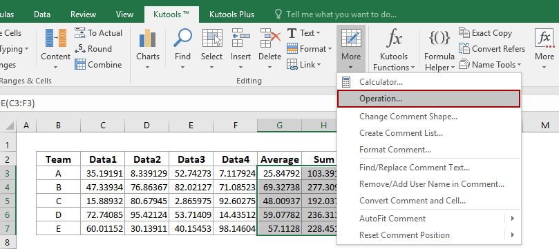
1. เลือกเซลล์สูตรที่คุณต้อง จำกัด ตำแหน่งทศนิยมแล้วคลิก Kutools > More > การดำเนินการ.

2. ในกล่องโต้ตอบ Operation Tools โปรดคลิกเพื่อไฮไลต์ การล้อม ใน การดำเนินการ กล่องรายการพิมพ์จำนวนตำแหน่งทศนิยมใน ตัวดำเนินการ และตรวจสอบส่วน สร้างสูตร ตัวเลือก
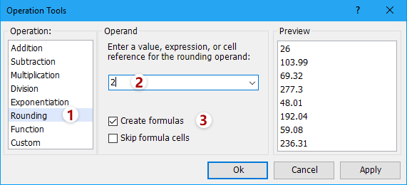
3. คลิก Ok ปุ่ม

ตอนนี้คุณจะเห็นเซลล์สูตรทั้งหมดถูกปัดเศษเป็นทศนิยมที่ระบุจำนวนมาก ดูภาพหน้าจอ:

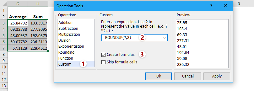
ปลาย: ถ้าคุณต้องการปัดเศษลงหรือปัดเศษเซลล์สูตรหลายเซลล์เป็นกลุ่มคุณสามารถตั้งค่าได้ดังนี้: ในกล่องโต้ตอบเครื่องมือการทำงาน (1) เลือก ประเพณี ในกล่องรายการการดำเนินการ (2) ชนิด = รอบ (?, 2) or = รอบลง (?, 2) ใน ประเพณี ส่วนและ (3) ตรวจสอบ สร้างสูตร ตัวเลือก ดูภาพหน้าจอ:


จำกัด จำนวนตำแหน่งทศนิยมในหลาย ๆ สูตรใน Excel ได้อย่างง่ายดาย

โดยปกติคุณลักษณะทศนิยมสามารถลดตำแหน่งทศนิยมในเซลล์ได้ แต่ค่าจริงที่แสดงในแถบสูตรจะไม่เปลี่ยนแปลงเลย Kutools สำหรับ Excel's รอบ ยูทิลิตี้สามารถช่วยคุณปัดเศษขึ้น / ลง / ถึงจุดทศนิยมที่ระบุได้อย่างง่ายดาย

Kutools สำหรับ Excel- รวมเครื่องมือที่มีประโยชน์มากกว่า 300 รายการสำหรับ Excel ทดลองใช้ฟรี 60 วันเต็มไม่ต้องใช้บัตรเครดิต! Get It Now

วิธีนี้จะปัดเศษเซลล์สูตรตามจำนวนตำแหน่งทศนิยมที่ระบุจำนวนมาก อย่างไรก็ตามจะลบสูตรออกจากเซลล์สูตรเหล่านี้และยังคงเป็นผลลัพธ์การปัดเศษเท่านั้น


Demo: จำกัด จำนวนตำแหน่งทศนิยมในสูตรใน Excel

Kutools สำหรับ Excel: เครื่องมือแสนสะดวกกว่า 300 รายการอยู่แค่เพียงปลายนิ้วสัมผัส! เริ่มทดลองใช้ฟรี 30 วันโดยไม่มีข้อจำกัดด้านฟีเจอร์ตั้งแต่วันนี้ Download Now!

บทความที่เกี่ยวข้อง:

สุดยอดเครื่องมือเพิ่มผลผลิตในสำนักงาน

🤖 Kutools AI ผู้ช่วย: ปฏิวัติการวิเคราะห์ข้อมูลโดยยึดตาม: การดำเนินการที่ชาญฉลาด   |  สร้างรหัส  |  สร้างสูตรที่กำหนดเอง  |  วิเคราะห์ข้อมูลและสร้างแผนภูมิ  |  เรียกใช้ฟังก์ชัน Kutools...
คุณสมบัติยอดนิยม: ค้นหา เน้น หรือระบุรายการที่ซ้ำกัน   |  ลบแถวว่าง   |  รวมคอลัมน์หรือเซลล์โดยไม่สูญเสียข้อมูล   |   รอบโดยไม่มีสูตร ...
การค้นหาขั้นสูง: VLookup หลายเกณฑ์    VLookup หลายค่า  |   VLookup ข้ามหลายแผ่น   |   การค้นหาที่ไม่ชัดเจน ....
รายการแบบเลื่อนลงขั้นสูง: สร้างรายการแบบหล่นลงอย่างรวดเร็ว   |  รายการแบบหล่นลงขึ้นอยู่กับ   |  เลือกหลายรายการแบบหล่นลง ....
ผู้จัดการคอลัมน์: เพิ่มจำนวนคอลัมน์เฉพาะ  |  ย้ายคอลัมน์  |  สลับสถานะการมองเห็นของคอลัมน์ที่ซ่อนอยู่  |  เปรียบเทียบช่วงและคอลัมน์ ...
คุณสมบัติเด่น: กริดโฟกัส   |  มุมมองการออกแบบ   |   บาร์สูตรใหญ่    สมุดงานและตัวจัดการชีต   |  ห้องสมุดทรัพยากร (ข้อความอัตโนมัติ)   |  เลือกวันที่   |  รวมแผ่นงาน   |  เข้ารหัส/ถอดรหัสเซลล์    ส่งอีเมลตามรายการ   |  ซุปเปอร์ฟิลเตอร์   |   ตัวกรองพิเศษ (กรองตัวหนา/ตัวเอียง/ขีดทับ...) ...
ชุดเครื่องมือ 15 อันดับแรก12 ข้อความ เครื่องมือ (เพิ่มข้อความ, ลบอักขระ, ... )   |   50 + แผนภูมิ ประเภท (แผนภูมิ Gantt, ... )   |   40+ ใช้งานได้จริง สูตร (คำนวณอายุตามวันเกิด, ... )   |   19 การแทรก เครื่องมือ (ใส่ QR Code, แทรกรูปภาพจากเส้นทาง, ... )   |   12 การแปลง เครื่องมือ (ตัวเลขเป็นคำ, การแปลงสกุลเงิน, ... )   |   7 ผสานและแยก เครื่องมือ (แถวรวมขั้นสูง, แยกเซลล์, ... )   |   ... และอื่น ๆ

เพิ่มพูนทักษะ Excel ของคุณด้วย Kutools สำหรับ Excel และสัมผัสประสิทธิภาพอย่างที่ไม่เคยมีมาก่อน Kutools สำหรับ Excel เสนอคุณสมบัติขั้นสูงมากกว่า 300 รายการเพื่อเพิ่มประสิทธิภาพและประหยัดเวลา  คลิกที่นี่เพื่อรับคุณสมบัติที่คุณต้องการมากที่สุด...

รายละเอียด


แท็บ Office นำอินเทอร์เฟซแบบแท็บมาที่ Office และทำให้งานของคุณง่ายขึ้นมาก

  • เปิดใช้งานการแก้ไขและอ่านแบบแท็บใน Word, Excel, PowerPoint, ผู้จัดพิมพ์, Access, Visio และโครงการ
  • เปิดและสร้างเอกสารหลายรายการในแท็บใหม่ของหน้าต่างเดียวกันแทนที่จะเป็นในหน้าต่างใหม่
  • เพิ่มประสิทธิภาพการทำงานของคุณ 50% และลดการคลิกเมาส์หลายร้อยครั้งให้คุณทุกวัน!
Comments (15)
No ratings yet. Be the first to rate!
This comment was minimized by the moderator on the site
this cnu
am using excel fo milk calculations

in 1 crate having 12/lit of milk.
if customar take 12/lit in total it shows 1 using,(=number1/number2)
if customar take 24/ in total it shows 2 using,(=number1/number2)
if customar take 36/ total it shows 3using,(=number1/number2)
but some customar take 15 or 22 or 35

if customar take 15 in total it shows 1.3
if customar take 22 in total it shows 1.10
if customar take35 in total it shows 2.11

i need formula for above calculation
This comment was minimized by the moderator on the site
try this:
=roundup(number1/number2,0)
This comment was minimized by the moderator on the site
'95,954,691.3389700060
When a put this data on excel, and quit the ' to turn it a number, excel, trucante the number after 5 decimal. The new number is 95,954,691.33897, but I need 10 decimals. How to resolve this?
This comment was minimized by the moderator on the site
Try this:

=TEXT(95954691.3389100060,"00,000,000.0000000000")
This comment was minimized by the moderator on the site
Ok, here is one I really need help with since it would ease my job a lot. I have a table where i need most of my cells to have 2 decimals. One of the columns (lets say C) has to be A multiplied by B, but with a little text following the result of the multiplication, hence i gave it a:
A*B & "text" formula
My problem is that if result of A*B is 3 or 3.1 it will appear just like that: "3 text" or "3.1 text", but i really need it as "3.00 text"/ "3.10text".
Any tips?
This comment was minimized by the moderator on the site
Try this:

=TEXT(A*B,"0.00")&" text"
This comment was minimized by the moderator on the site
I want to set a limit whereas 0.60 is the threshold if the decimal reaches 0.60 it will automatically count as 1 and reset into decimal. The decimal represent the minutes and the whole number represent the hours. I'm presenting my data as numbers instead of timevalue. Hope anyone can help
This comment was minimized by the moderator on the site
Unfortunately it is not working if you concatenate:

I want to combine two cells A and B with many digits to A (B) with onlytwo digits.

I tried like that:
=CONCATENATE((ROUND(C4,1))," (",(Round(D4,1)),")")

It doesn't work and shows only the formula.
Can anyone help?
This comment was minimized by the moderator on the site
Hi yvonne Fabian,
Your formula works well in my Excel 2016.
This comment was minimized by the moderator on the site
how to deal with two decimal points e.g. 138.4622.472, 137.1416.113 etc. any way to get rid of .472 and .113 and so on
This comment was minimized by the moderator on the site
John, to round to 0 decimals, try use ROUND(CELL,0) and to round DOWN to the number, use INT (integer).
ROUND(12.5,0) = 13 ; INT(12.5) = 12
for the same but not to whole number but e.g. tenths, first multiply the baste number by 10, then ROUND/INT and then devide back by ten.
This comment was minimized by the moderator on the site
Here we are inserting the values in one cell(A1) and applying the formula in another cell(D1) (for example) and in that cell(D1) only we are getting the output , but I want to apply the formula in cell(A1) only so I can get the output in that cell (A1).
If I am doing this then I am not getting any output in the cell (A1).
Please help me to achieve this.
This comment was minimized by the moderator on the site
Hi Narsingh,
Kutools for Excel provides an Operation tools which can custom formula to selected cells. This feature may solve your problem.
This comment was minimized by the moderator on the site
Here we are inserting the values in one cell(A1) and applying the formula in another cell(D1) (for example) and in that cell(D1) only we are getting the output , but I want to apply the formula in cell(A1) only so I can get the output in that cell (A1).
If I am doing this then I am not getting any output in the cell (A1).
Please help me to achieve this.
This comment was minimized by the moderator on the site
thanks, this soo helpfull :-)
There are no comments posted here yet
Please leave your comments in English
Posting as Guest
×
Rate this post:
0   Characters
Suggested Locations