ไปยังเนื้อหาหลัก

วิธีแยกค่าที่ไม่ซ้ำจากหลายคอลัมน์ใน Excel

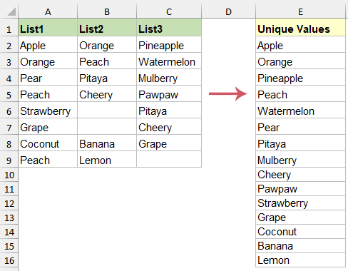
สมมติว่าคุณมีหลายคอลัมน์ที่มีหลายค่าค่าบางค่าจะซ้ำกันในคอลัมน์เดียวกันหรือคนละคอลัมน์ และตอนนี้คุณต้องการค้นหาค่าที่มีอยู่ในคอลัมน์ใดคอลัมน์หนึ่งเพียงครั้งเดียว มีเคล็ดลับง่ายๆสำหรับคุณในการดึงค่าที่ไม่ซ้ำกันจากหลายคอลัมน์ใน Excel หรือไม่?


แยกค่าที่ไม่ซ้ำจากหลายคอลัมน์ด้วยสูตร

ส่วนนี้จะครอบคลุมถึงสองสูตร: สูตรหนึ่งใช้สูตรอาร์เรย์ที่เหมาะสำหรับ Excel เวอร์ชันทั้งหมด และอีกสูตรหนึ่งใช้สูตรอาร์เรย์แบบไดนามิกสำหรับ Excel 365 โดยเฉพาะ

แยกค่าที่ไม่ซ้ำจากหลายคอลัมน์ด้วยสูตร Array สำหรับ Excel เวอร์ชันทั้งหมด

สำหรับผู้ใช้ที่มี Excel เวอร์ชันใดก็ตาม สูตรอาร์เรย์สามารถเป็นเครื่องมือที่มีประสิทธิภาพในการแยกค่าที่ไม่ซ้ำกันจากหลายคอลัมน์ ต่อไปนี้คือวิธีที่คุณสามารถทำได้:

1. สมมติว่าค่าของคุณอยู่ในช่วง A2: C9โปรดป้อนสูตรต่อไปนี้ลงในเซลล์ E2:

=INDIRECT(TEXT(MIN(IF(($A$2:$C$9<>"")*(COUNTIF($E$1:E1,$A$2:$C$9)=0),ROW($2:$9)*100+COLUMN($A:$C),7^8)),"R0C00"),)&""
หมายเหตุ: ในสูตรข้างต้น A2: C9 ระบุช่วงของเซลล์ที่คุณต้องการดึงค่าเฉพาะ E1: E1 คือเซลล์แรกของคอลัมน์ที่คุณต้องการวางผลลัพธ์ $ 2: $ 9 แถวนั้นมีเซลล์ที่คุณต้องการใช้และ $ A: $ C ระบุว่าคอลัมน์มีเซลล์ที่คุณต้องการใช้ โปรดเปลี่ยนเป็นของคุณเอง

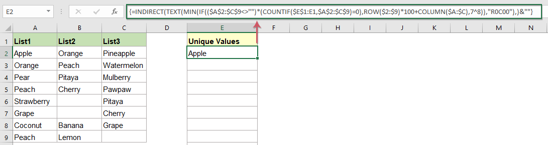
2. จากนั้นกด Shift + Ctrl + Enter เข้าด้วยกันจากนั้นลากจุดจับเติมเพื่อแยกค่าที่ไม่ซ้ำกันจนกว่าเซลล์ว่างจะปรากฏขึ้น ดูภาพหน้าจอ:

คำอธิบายของสูตรนี้:
  1. $ ก $ 2: $ C $ 9: ระบุช่วงข้อมูลที่จะตรวจสอบ ซึ่งก็คือเซลล์ตั้งแต่ A2 ถึง C9
  2. IF(($A$2:$C$9<>"")*(COUNTIF($E$1:E1,$A$2:$C$9)=0), ROW($2:$9)*100+COLUMN($A:$C), 7^8):
    • $A$2:$C$9<>"" ตรวจสอบว่าเซลล์ในช่วงไม่ว่างเปล่าหรือไม่
    • COUNTIF($E$1:E1,$A$2:$C$9)=0 กำหนดว่าค่าของเซลล์เหล่านี้ยังไม่ได้แสดงอยู่ในช่วงของเซลล์ตั้งแต่ E1 ถึง E1
    • หากตรงตามเงื่อนไขทั้งสอง (เช่น ค่าไม่ว่างเปล่าและยังไม่ได้แสดงอยู่ในคอลัมน์ E) ฟังก์ชัน IF จะคำนวณตัวเลขที่ไม่ซ้ำกันตามแถวและคอลัมน์ (ROW($2:$9)*100+COLUMN($A: $ซี)).
    • ถ้าไม่ตรงตามเงื่อนไข ฟังก์ชันจะส่งกลับตัวเลขจำนวนมาก (7^8) ซึ่งทำหน้าที่เป็นตัวยึดตำแหน่ง
  3. นาที(...): ค้นหาตัวเลขที่น้อยที่สุดที่ส่งคืนโดยฟังก์ชัน IF ด้านบน ซึ่งสอดคล้องกับตำแหน่งของค่าที่ไม่ซ้ำถัดไป
  4. ข้อความ(...,"R0C00"): แปลงตัวเลขขั้นต่ำนี้เป็นที่อยู่สไตล์ R1C1 รหัสรูปแบบ R0C00 ระบุการแปลงตัวเลขเป็นรูปแบบการอ้างอิงเซลล์ Excel
  5. ทางอ้อม(...): ใช้ฟังก์ชัน INDIRECT เพื่อแปลงที่อยู่สไตล์ R1C1 ที่สร้างในขั้นตอนก่อนหน้ากลับไปเป็นการอ้างอิงเซลล์สไตล์ A1 ปกติ ฟังก์ชัน INDIRECT ช่วยให้สามารถอ้างอิงเซลล์ตามเนื้อหาของสตริงข้อความ
  6. &"": การต่อท้าย &"" ที่ส่วนท้ายของสูตรทำให้มั่นใจได้ว่าเอาต์พุตสุดท้ายจะถือเป็นข้อความ ดังนั้นเลขคู่จึงจะแสดงเป็นข้อความ
 
แยกค่าที่ไม่ซ้ำจากหลายคอลัมน์ด้วยสูตรสำหรับ Excel 365

Excel 365 รองรับอาร์เรย์แบบไดนามิก ทำให้ง่ายต่อการแยกค่าที่ไม่ซ้ำจากหลายคอลัมน์:

โปรดป้อนหรือคัดลอกสูตรต่อไปนี้ลงในเซลล์ว่างที่คุณต้องการใส่ผลลัพธ์ จากนั้นคลิก เข้าสู่ กุญแจสำคัญในการรับค่าที่ไม่ซ้ำทั้งหมดพร้อมกัน ดูภาพหน้าจอ:

=UNIQUE(TOCOL(A2:C9,1))


แยกค่าที่ไม่ซ้ำจากหลายคอลัมน์ด้วย Kutools AI Aide

ปลดปล่อยพลังของ Kutools AI ผู้ช่วย เพื่อแยกค่าที่ไม่ซ้ำจากหลายคอลัมน์ใน Excel ได้อย่างราบรื่น ด้วยการคลิกเพียงไม่กี่ครั้ง เครื่องมืออัจฉริยะนี้จะกรองข้อมูลของคุณ ระบุและแสดงรายการที่ไม่ซ้ำกันในช่วงที่เลือก ลืมความยุ่งยากของสูตรที่ซับซ้อนหรือโค้ด vba ไปได้เลย ยอมรับประสิทธิภาพของ Kutools AI ผู้ช่วย และเปลี่ยนเวิร์กโฟลว์ Excel ของคุณให้เป็นประสบการณ์ที่มีประสิทธิผลและปราศจากข้อผิดพลาดมากขึ้น

หมายเหตุ: หากต้องการใช้สิ่งนี้ Kutools AI ผู้ช่วย of Kutools สำหรับ Excelโปรด ดาวน์โหลดและติดตั้ง Kutools สำหรับ Excel ก่อน

หลังจากติดตั้ง Kutools for Excel แล้วโปรดคลิก Kutools AI > เอไอ ผู้ช่วย เพื่อเปิด Kutools AI ผู้ช่วย บานหน้าต่าง:

  1. พิมพ์ความต้องการของคุณลงในกล่องแชทแล้วคลิก ส่ง หรือกด เข้าสู่ กุญแจสำคัญในการส่งคำถาม
    "แยกค่าที่ไม่ซ้ำออกจากช่วง A2:C9 โดยไม่สนใจเซลล์ว่าง และวางผลลัพธ์โดยเริ่มต้นที่ E2:"
  2. หลังจากวิเคราะห์แล้วคลิก ดำเนินงาน ปุ่มเพื่อเรียกใช้ Kutools AI Aide จะประมวลผลคำขอของคุณโดยใช้ AI และส่งคืนผลลัพธ์ในเซลล์ที่ระบุโดยตรงใน Excel


แยกค่าที่ไม่ซ้ำกันจากหลายคอลัมน์ด้วย Pivot Table

หากคุณคุ้นเคยกับตาราง Pivot คุณสามารถแยกค่าที่ไม่ซ้ำกันออกจากคอลัมน์หลายคอลัมน์โดยทำตามขั้นตอนต่อไปนี้:

1. ในตอนแรกโปรดแทรกคอลัมน์ว่างใหม่ทางด้านซ้ายของข้อมูลในตัวอย่างนี้ฉันจะแทรกคอลัมน์ A ข้างข้อมูลต้นฉบับ

2. คลิกเซลล์หนึ่งเซลล์ในข้อมูลของคุณแล้วกด Alt + D จากนั้นกด P ทันทีเพื่อเปิดไฟล์ PivotTable และ PivotChart Wizardเลือก ช่วงการรวมหลายรายการ ในวิซาร์ด step1 ดูภาพหน้าจอ:

3. จากนั้นคลิก ถัดไป ปุ่มตรวจสอบ สร้างฟิลด์หน้าเดียวให้ฉัน ตัวเลือกในวิซาร์ด step2 ดูภาพหน้าจอ:

4. ไปที่การคลิก ถัดไป คลิกเพื่อเลือกช่วงข้อมูลซึ่งรวมคอลัมน์ใหม่ทางซ้ายของเซลล์จากนั้นคลิก เพิ่ม เพื่อเพิ่มช่วงข้อมูลลงในไฟล์ ทุกช่วง กล่องรายการดูภาพหน้าจอ:

5. หลังจากเลือกช่วงข้อมูลแล้วให้คลิกต่อ ถัดไปในวิซาร์ดขั้นตอนที่ 3 ให้เลือกตำแหน่งที่คุณต้องการวางรายงาน PivotTable ตามที่คุณต้องการ

6. ในที่สุดคลิก เสร็จสิ้น เพื่อทำวิซาร์ดให้เสร็จสมบูรณ์และมีการสร้างตาราง Pivot ในแผ่นงานปัจจุบันจากนั้นยกเลิกการเลือกฟิลด์ทั้งหมดจาก เลือกช่องที่จะเพิ่มในรายงาน ส่วนดูภาพหน้าจอ:

7. จากนั้นตรวจสอบฟิลด์ ความคุ้มค่า หรือลากค่าไปที่ แถว ตอนนี้คุณจะได้รับค่าที่ไม่ซ้ำกันจากหลายคอลัมน์ดังนี้:


แยกค่าที่ไม่ซ้ำกันจากหลายคอลัมน์ด้วยรหัส VBA

ด้วยรหัส VBA ต่อไปนี้คุณยังสามารถแยกค่าที่ไม่ซ้ำกันจากหลายคอลัมน์ได้

1. กด ALT + F11 และจะเปิดไฟล์ หน้าต่าง Microsoft Visual Basic for Applications.

2. คลิก สิ่งที่ใส่เข้าไป > โมดูลและวางรหัสต่อไปนี้ในหน้าต่างโมดูล

VBA: ดึงค่าที่ไม่ซ้ำกันจากหลายคอลัมน์

Sub Uniquedata()
'Updateby Extendoffice
Dim rng As Range
Dim InputRng As Range, OutRng As Range
Set dt = CreateObject("Scripting.Dictionary")
xTitleId = "KutoolsforExcel"
Set InputRng = Application.Selection
Set InputRng = Application.InputBox("Range :", xTitleId, InputRng.Address, Type:=8)
Set OutRng = Application.InputBox("Out put to (single cell):", xTitleId, Type:=8)
For Each rng In InputRng
    If rng.Value <> "" Then
        dt(rng.Value) = ""
    End If
Next
OutRng.Range("A1").Resize(dt.Count) = Application.WorksheetFunction.Transpose(dt.Keys)
End Sub

3. จากนั้นกด F5 เพื่อเรียกใช้รหัสนี้และกล่องพร้อมต์จะปรากฏขึ้นเพื่อเตือนให้คุณเลือกช่วงข้อมูลที่คุณต้องการใช้ ดูภาพหน้าจอ:

4. จากนั้นคลิก OKกล่องข้อความแจ้งอีกอันจะปรากฏขึ้นเพื่อให้คุณเลือกสถานที่ที่จะใส่ผลลัพธ์ดูภาพหน้าจอ:

5. คลิก OK เพื่อปิดกล่องโต้ตอบนี้และค่าที่ไม่ซ้ำกันทั้งหมดจะถูกแยกออกพร้อมกัน


บทความที่เกี่ยวข้องเพิ่มเติม:

  • นับจำนวนค่าที่เป็นเอกลักษณ์และแตกต่างจากรายการ
  • สมมติว่าคุณมีรายการค่าที่ยาวพร้อมกับรายการที่ซ้ำกันบางรายการตอนนี้คุณต้องการนับจำนวนค่าที่ไม่ซ้ำกัน (ค่าที่ปรากฏในรายการเพียงครั้งเดียว) หรือค่าที่ไม่ซ้ำกัน (ค่าที่แตกต่างกันทั้งหมดในรายการหมายความว่าไม่ซ้ำกัน ค่า + ค่าที่ซ้ำกันครั้งที่ 1) ในคอลัมน์ตามภาพหน้าจอด้านซ้ายที่แสดง บทความนี้ฉันจะพูดถึงวิธีจัดการกับงานนี้ใน Excel
  • แยกค่าที่ไม่ซ้ำกันตามเกณฑ์ใน Excel
  • สมมติว่าคุณมีช่วงข้อมูลต่อไปนี้ที่คุณต้องการแสดงเฉพาะชื่อเฉพาะของคอลัมน์ B ตามเกณฑ์เฉพาะของคอลัมน์ A เพื่อให้ได้ผลลัพธ์ตามภาพด้านล่างที่แสดง คุณจะจัดการกับงานนี้ใน Excel อย่างรวดเร็วและง่ายดายได้อย่างไร?
  • อนุญาตเฉพาะค่าที่ไม่ซ้ำใน Excel
  • หากคุณต้องการเก็บเฉพาะค่าที่ไม่ซ้ำกันเท่านั้นที่ป้อนในคอลัมน์ของแผ่นงานและป้องกันไม่ให้ซ้ำกันบทความนี้จะแนะนำเคล็ดลับง่ายๆสำหรับคุณในการจัดการกับงานนี้
  • รวมค่าที่ไม่ซ้ำกันตามเกณฑ์ใน Excel
  • ตัวอย่างเช่นฉันมีช่วงของข้อมูลที่มีคอลัมน์ชื่อและลำดับในขณะนี้เพื่อรวมเฉพาะค่าที่ไม่ซ้ำกันในคอลัมน์คำสั่งซื้อตามคอลัมน์ชื่อตามภาพหน้าจอต่อไปนี้ วิธีแก้ปัญหานี้อย่างรวดเร็วและง่ายดายใน Excel

สุดยอดเครื่องมือเพิ่มผลผลิตในสำนักงาน

🤖 Kutools AI ผู้ช่วย: ปฏิวัติการวิเคราะห์ข้อมูลโดยยึดตาม: การดำเนินการที่ชาญฉลาด   |  สร้างรหัส  |  สร้างสูตรที่กำหนดเอง  |  วิเคราะห์ข้อมูลและสร้างแผนภูมิ  |  เรียกใช้ฟังก์ชัน Kutools...
คุณสมบัติยอดนิยม: ค้นหา เน้น หรือระบุรายการที่ซ้ำกัน   |  ลบแถวว่าง   |  รวมคอลัมน์หรือเซลล์โดยไม่สูญเสียข้อมูล   |   รอบโดยไม่มีสูตร ...
การค้นหาขั้นสูง: VLookup หลายเกณฑ์    VLookup หลายค่า  |   VLookup ข้ามหลายแผ่น   |   การค้นหาที่ไม่ชัดเจน ....
รายการแบบเลื่อนลงขั้นสูง: สร้างรายการแบบหล่นลงอย่างรวดเร็ว   |  รายการแบบหล่นลงขึ้นอยู่กับ   |  เลือกหลายรายการแบบหล่นลง ....
ผู้จัดการคอลัมน์: เพิ่มจำนวนคอลัมน์เฉพาะ  |  ย้ายคอลัมน์  |  สลับสถานะการมองเห็นของคอลัมน์ที่ซ่อนอยู่  |  เปรียบเทียบช่วงและคอลัมน์ ...
คุณสมบัติเด่น: กริดโฟกัส   |  มุมมองการออกแบบ   |   บาร์สูตรใหญ่    สมุดงานและตัวจัดการชีต   |  ห้องสมุดทรัพยากร (ข้อความอัตโนมัติ)   |  เลือกวันที่   |  รวมแผ่นงาน   |  เข้ารหัส/ถอดรหัสเซลล์    ส่งอีเมลตามรายการ   |  ซุปเปอร์ฟิลเตอร์   |   ตัวกรองพิเศษ (กรองตัวหนา/ตัวเอียง/ขีดทับ...) ...
ชุดเครื่องมือ 15 อันดับแรก12 ข้อความ เครื่องมือ (เพิ่มข้อความ, ลบอักขระ, ... )   |   50 + แผนภูมิ ประเภท (แผนภูมิ Gantt, ... )   |   40+ ใช้งานได้จริง สูตร (คำนวณอายุตามวันเกิด, ... )   |   19 การแทรก เครื่องมือ (ใส่ QR Code, แทรกรูปภาพจากเส้นทาง, ... )   |   12 การแปลง เครื่องมือ (ตัวเลขเป็นคำ, การแปลงสกุลเงิน, ... )   |   7 ผสานและแยก เครื่องมือ (แถวรวมขั้นสูง, แยกเซลล์, ... )   |   ... และอื่น ๆ

เพิ่มพูนทักษะ Excel ของคุณด้วย Kutools สำหรับ Excel และสัมผัสประสิทธิภาพอย่างที่ไม่เคยมีมาก่อน Kutools สำหรับ Excel เสนอคุณสมบัติขั้นสูงมากกว่า 300 รายการเพื่อเพิ่มประสิทธิภาพและประหยัดเวลา  คลิกที่นี่เพื่อรับคุณสมบัติที่คุณต้องการมากที่สุด...

รายละเอียด


แท็บ Office นำอินเทอร์เฟซแบบแท็บมาที่ Office และทำให้งานของคุณง่ายขึ้นมาก

  • เปิดใช้งานการแก้ไขและอ่านแบบแท็บใน Word, Excel, PowerPoint, ผู้จัดพิมพ์, Access, Visio และโครงการ
  • เปิดและสร้างเอกสารหลายรายการในแท็บใหม่ของหน้าต่างเดียวกันแทนที่จะเป็นในหน้าต่างใหม่
  • เพิ่มประสิทธิภาพการทำงานของคุณ 50% และลดการคลิกเมาส์หลายร้อยครั้งให้คุณทุกวัน!
Comments (31)
Rated 5 out of 5 · 1 ratings
This comment was minimized by the moderator on the site
Thank you for this solution, however what if the columns are in separate excel sheet? or is in separate columns instead of a table?
This comment was minimized by the moderator on the site
Hello, Jon,
The methods in this article ar only works well for a range of data, if your data in separate columns, you should copy and paste them into one range first, and then apply the formula or VBA code.
Thank you!
This comment was minimized by the moderator on the site
Thank you for this great article.

For people who are using the array formular in non-English Excel there must be taken special care of the text format string: in your example: "R0C00".
For German this would translate to "Z0S00". However, "S" is a special character refering to seconds for time formating. This character needs to be escaped and therefore the correct format string for German Excel is "Z0\S00".

I hope this helps someone in the future :-)
This comment was minimized by the moderator on the site
Hello, Michael H.
Thanks for your kindly explanation.
Hope this can help others in the future.😄
This comment was minimized by the moderator on the site
Thank you for this great article.

For people who are using the array formular in non-English Excel there must be taken special care of the text format string: in your example: "R0C00".
For German this would translate to "Z0S00". However, "S" is a special character refering to seconds for time formating. This character needs to be escaped and therefore the correct format string for German Excel is "Z0\S00".

I hope this helps someone in the future :-)
This comment was minimized by the moderator on the site
Hello Sir! The VBA worked wonders, thank you very much for that! I was wondering, If I change the original data, is it possible to refresh the column with the unique values automatically?
Rated 5 out of 5
This comment was minimized by the moderator on the site
Hello Ioannis,

Glad to help. After you change the original data, the VBA can not refresh the result automatically. And the easiest way I can think of is to press Ctrl + Alt + F9 to refresh all results in worksheets in all open workbooks. Have a nice day.

Sincerely,
Mandy
This comment was minimized by the moderator on the site
The array formula at the top is working great when used with data in the same sheet, however when I try to use it to reference the same exact data from another sheet the formula returns nothing. I'm unable to figure out why. Is there a limitation with array functions that prevents you from referencing ranges in a different sheet?

Thanks for any insight you can provide.
This comment was minimized by the moderator on the site
Hello Erin,

Glad to help. The INDIRECT function in this formula is more complicated to use when referencing data in other worksheets. It is not recommended to use this feature when referencing ranges in different worksheets.

For example: Now the data is in Sheet1, I want to reference the content of cell C2 of Sheet1 in Sheet2. First, in any two cells in Sheet2, such as D1 and D2, enter Sheet1 and C2, respectively. At this point, enter the formula in the empty cell of Sheet2:
=INDIRECT("'"&D1&"'!"&D2), then the content of cell C2 in Sheet1 can be returned.

As you can see, it make things way more complex. Hope my explanation can help. Have a nice day.

Sincerely,
Mandy
This comment was minimized by the moderator on the site
Czy to żart?
This comment was minimized by the moderator on the site
can we create uniqdata function instead of macro?
This comment was minimized by the moderator on the site
Hi, İlhan,If you like a User Defined Function to create a formula for solving this problem, the below code may help you:After inserting the code, select a list of cells where you want to put the results. Then type this formula:=Uniques(A1:C4)  in the formula bar.Press Ctrl+Shift+Enter keys together. 


Function Uniques(ByVal inputRange As Range)
Dim inputArray As Variant
Dim myColl As New Collection
Dim xVal As Variant
Dim outArray() As Variant
On Error Resume Next
With inputRange
inputArray = Application.Intersect(.Cells, .Parent.UsedRange).Value
End With
On Error GoTo 0
On Error Resume Next
For Each xVal In inputArray
myColl.*** Item:=xVal, Key:=(CStr(xVal) & TypeName(xVal))
Next xVal
myColl.Remove "String"
On Error GoTo 0
ReDim outArray(1 To Application.Max(myColl.Count, Application.Caller.Cells.Count))
For xVal = 1 To UBound(outArray)
outArray(xVal) = vbNullString
Next xVal
For xVal = 1 To Application.Min(myColl.Count, Application.Caller.Cells.Count)
outArray(xVal) = myColl(xVal)
Next xVal
If Application.Caller.Columns.Count = 1 Then
Uniques = Application.Transpose(outArray)
Else
Uniques = outArray
End If
End Function
This comment was minimized by the moderator on the site
Thanks for the code. I'm using the VBA code of this page. Is there a way to add a sorting code after the unique values are extracted so it sorts it automatically?
This comment was minimized by the moderator on the site
Regarding the formula version, could you explain in more detail what this portion is doing? *100+COLUMN($A:$C),7^8)),"R0C00") Specifically, what are the *100, 7^8, and "R0C000" doing? I'm understanding everything else, but I can't figure out what these are for.
This comment was minimized by the moderator on the site
Little late for my response here but...
ROW($2:$9)*100 - this is multiplying the row number *100, so if it's in row 5, now the number is 500
COLUMN($A:$C) - this gets added to the row*100 number, so if it's row 5 col 2, then the number is 502.
7^8)), - this (I think) is to have a max value for the min statement from earlier.
"R0C00") - this formats the text based on the number. In the example, we had 502 so this gives R5C02 (row 5, col 02).

If you have a lot of columns but not many rows, then you could change it to ROW($2:$9)*1000+COLUMN($A:$C),7^8)),"R0C000")
This comment was minimized by the moderator on the site
i've adjusted to my sheet but am only returning the first value in the defined array... what am i missing?
This comment was minimized by the moderator on the site
Hello, Cody,
The above formula works well in my worksheet, could you give a screenshot of your data problem here?
Thank you!
There are no comments posted here yet
Load More
Please leave your comments in English
Posting as Guest
×
Rate this post:
0   Characters
Suggested Locations