ไปยังเนื้อหาหลัก

วิธีแยกค่าที่ไม่ซ้ำตามเกณฑ์ใน Excel

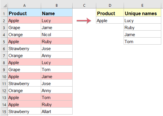
สมมติว่าคุณมีช่วงข้อมูลด้านซ้ายที่คุณต้องการแสดงเฉพาะชื่อเฉพาะของคอลัมน์ B ตามเกณฑ์เฉพาะของคอลัมน์ A เพื่อให้ได้ผลลัพธ์ตามภาพด้านล่างที่แสดง คุณจะจัดการกับงานนี้ใน Excel อย่างรวดเร็วและง่ายดายได้อย่างไร?

แยกค่าที่ไม่ซ้ำกันตามเกณฑ์ด้วยสูตรอาร์เรย์

แยกค่าที่ไม่ซ้ำกันตามเกณฑ์หลายเกณฑ์ด้วยสูตรอาร์เรย์

ดึงค่าที่ไม่ซ้ำกันออกจากรายการเซลล์ด้วยคุณสมบัติที่มีประโยชน์


แยกค่าที่ไม่ซ้ำกันตามเกณฑ์ด้วยสูตรอาร์เรย์

ในการแก้ปัญหานี้คุณสามารถใช้สูตรอาร์เรย์ที่ซับซ้อนได้โปรดทำดังนี้:

1. ป้อนสูตรด้านล่างลงในเซลล์ว่างที่คุณต้องการแสดงรายการผลการแยกในตัวอย่างนี้ฉันจะใส่ลงในเซลล์ E2 จากนั้นกด Shift + Ctrl + Enter คีย์เพื่อรับค่าแรกที่ไม่ซ้ำกัน

=IFERROR(INDEX($B$2:$B$15, MATCH(0, IF($D$2=$A$2:$A$15, COUNTIF($E$1:$E1, $B$2:$B$15), ""), 0)),"")

2. จากนั้นลากที่จับเติมลงไปที่เซลล์จนกว่าเซลล์ว่างจะปรากฏขึ้นและตอนนี้ค่าที่ไม่ซ้ำกันทั้งหมดตามเกณฑ์เฉพาะได้รับการระบุไว้ดูภาพหน้าจอ:

หมายเหตุ ในสูตรข้างต้น: B2: B15 คือช่วงคอลัมน์มีค่าเฉพาะที่คุณต้องการดึงออกมา A2: A15 คือคอลัมน์มีเกณฑ์ที่คุณอ้างอิง D2 บ่งชี้เกณฑ์ที่คุณต้องการแสดงรายการค่าที่ไม่ซ้ำกันตามและ E1 คือเซลล์เหนือสูตรที่คุณป้อน

แยกค่าที่ไม่ซ้ำกันตามเกณฑ์หลายเกณฑ์ด้วยสูตรอาร์เรย์

หากคุณต้องการแยกค่าที่ไม่ซ้ำกันตามเงื่อนไขสองเงื่อนไขนี่คือสูตรอาร์เรย์อื่นที่สามารถช่วยคุณได้โปรดทำดังนี้

1. ป้อนสูตรด้านล่างลงในเซลล์ว่างที่คุณต้องการแสดงรายการค่าที่ไม่ซ้ำกันในตัวอย่างนี้ฉันจะใส่ลงในเซลล์ G2 แล้วกด Shift + Ctrl + Enter คีย์เพื่อรับค่าแรกที่ไม่ซ้ำกัน

=IFERROR(INDEX($C$2:$C$15,MATCH(0,COUNTIF(G1:$G$1,$C$2:$C$15)+IF($A$2:$A$15<>$E$2,1,0)+IF($B$2:$B$15<>$F$2,1,0),0)),"")

2. จากนั้นลากที่จับเติมลงไปที่เซลล์จนกว่าเซลล์ว่างจะปรากฏขึ้นและตอนนี้ค่าที่ไม่ซ้ำกันทั้งหมดตามเงื่อนไขสองเงื่อนไขที่ระบุได้รับการระบุไว้ดูภาพหน้าจอ:

หมายเหตุ ในสูตรข้างต้น: C2: C15 คือช่วงคอลัมน์มีค่าเฉพาะที่คุณต้องการดึงออกมา A2: A15 และ E2 เป็นช่วงแรกที่มีเกณฑ์ที่คุณต้องการดึงค่าที่ไม่ซ้ำกันตาม B2: B15 และ F2 เป็นช่วงที่สองที่มีเกณฑ์ที่คุณต้องการดึงค่าที่ไม่ซ้ำกันตามและ G1 คือเซลล์เหนือสูตรที่คุณป้อน

ดึงค่าที่ไม่ซ้ำกันออกจากรายการเซลล์ด้วยคุณสมบัติที่มีประโยชน์

บางครั้งคุณแค่ต้องการดึงค่าที่ไม่ซ้ำกันออกจากรายการเซลล์ที่นี่ฉันจะแนะนำเครื่องมือที่มีประโยชน์ -Kutools สำหรับ Excelเดียวกันกับที่ แยกเซลล์ด้วยค่าที่ไม่ซ้ำกัน (รวมรายการที่ซ้ำกันครั้งแรก) ยูทิลิตี้คุณสามารถดึงค่าเฉพาะได้อย่างรวดเร็ว

หมายเหตุที่จะใช้สิ่งนี้ แยกเซลล์ด้วยค่าที่ไม่ซ้ำกัน (รวมรายการที่ซ้ำกันครั้งแรก)ประการแรกคุณควรดาวน์โหลดไฟล์ Kutools สำหรับ Excelแล้วใช้คุณสมบัตินี้อย่างรวดเร็วและง่ายดาย

หลังจากการติดตั้ง Kutools สำหรับ Excelโปรดทำตามนี้:

1. คลิกเซลล์ที่คุณต้องการให้ผลลัพธ์ออกมา (หมายเหตุ: อย่าคลิกเซลล์ในแถวแรก)

2. จากนั้นคลิก Kutools > ตัวช่วยสูตร > ตัวช่วยสูตรดูภาพหน้าจอ:

3. ใน ตัวช่วยสูตร โปรดดำเนินการดังต่อไปนี้:

  • เลือก ข้อความ ตัวเลือกจาก สูตร ชนิดภาพเขียน รายการแบบหล่นลง
  • จากนั้นเลือก แยกเซลล์ด้วยค่าที่ไม่ซ้ำกัน (รวมรายการที่ซ้ำกันครั้งแรก) จาก เลือก fromula กล่องรายการ;
  • ทางด้านขวา การป้อนอาร์กิวเมนต์ เลือกรายการเซลล์ที่คุณต้องการแยกค่าที่ไม่ซ้ำกัน

4. จากนั้นคลิก Ok ผลลัพธ์แรกจะปรากฏในเซลล์จากนั้นเลือกเซลล์แล้วลากที่จับเติมไปยังเซลล์ที่คุณต้องการแสดงรายการค่าที่ไม่ซ้ำกันทั้งหมดจนกว่าเซลล์ว่างจะปรากฏขึ้นดูภาพหน้าจอ:

ดาวน์โหลด Kutools for Excel ได้ฟรีทันที!


บทความที่เกี่ยวข้องเพิ่มเติม:

  • นับจำนวนค่าที่เป็นเอกลักษณ์และแตกต่างจากรายการ
  • สมมติว่าคุณมีรายการค่าที่ยาวพร้อมกับรายการที่ซ้ำกันบางรายการตอนนี้คุณต้องการนับจำนวนค่าที่ไม่ซ้ำกัน (ค่าที่ปรากฏในรายการเพียงครั้งเดียว) หรือค่าที่ไม่ซ้ำกัน (ค่าที่แตกต่างกันทั้งหมดในรายการหมายความว่าไม่ซ้ำกัน ค่า + ค่าที่ซ้ำกันครั้งที่ 1) ในคอลัมน์ตามภาพหน้าจอด้านซ้ายที่แสดง บทความนี้ฉันจะพูดถึงวิธีจัดการกับงานนี้ใน Excel
  • รวมค่าที่ไม่ซ้ำกันตามเกณฑ์ใน Excel
  • ตัวอย่างเช่นฉันมีช่วงของข้อมูลที่มีคอลัมน์ชื่อและลำดับในขณะนี้เพื่อรวมเฉพาะค่าที่ไม่ซ้ำกันในคอลัมน์คำสั่งซื้อตามคอลัมน์ชื่อตามภาพหน้าจอต่อไปนี้ วิธีแก้ปัญหานี้อย่างรวดเร็วและง่ายดายใน Excel
  • เชื่อมต่อค่าที่ไม่ซ้ำกันใน Excel
  • ถ้าฉันมีรายการค่าที่ยาวซึ่งเติมด้วยข้อมูลที่ซ้ำกันบางค่าตอนนี้ฉันต้องการค้นหาเฉพาะค่าที่ไม่ซ้ำกันแล้วรวมเข้าด้วยกันเป็นเซลล์เดียว ฉันจะจัดการกับปัญหานี้อย่างรวดเร็วและง่ายดายใน Excel ได้อย่างไร

สุดยอดเครื่องมือเพิ่มผลผลิตในสำนักงาน

🤖 Kutools AI ผู้ช่วย: ปฏิวัติการวิเคราะห์ข้อมูลโดยยึดตาม: การดำเนินการที่ชาญฉลาด   |  สร้างรหัส  |  สร้างสูตรที่กำหนดเอง  |  วิเคราะห์ข้อมูลและสร้างแผนภูมิ  |  เรียกใช้ฟังก์ชัน Kutools...
คุณสมบัติยอดนิยม: ค้นหา เน้น หรือระบุรายการที่ซ้ำกัน   |  ลบแถวว่าง   |  รวมคอลัมน์หรือเซลล์โดยไม่สูญเสียข้อมูล   |   รอบโดยไม่มีสูตร ...
การค้นหาขั้นสูง: VLookup หลายเกณฑ์    VLookup หลายค่า  |   VLookup ข้ามหลายแผ่น   |   การค้นหาที่ไม่ชัดเจน ....
รายการแบบเลื่อนลงขั้นสูง: สร้างรายการแบบหล่นลงอย่างรวดเร็ว   |  รายการแบบหล่นลงขึ้นอยู่กับ   |  เลือกหลายรายการแบบหล่นลง ....
ผู้จัดการคอลัมน์: เพิ่มจำนวนคอลัมน์เฉพาะ  |  ย้ายคอลัมน์  |  สลับสถานะการมองเห็นของคอลัมน์ที่ซ่อนอยู่  |  เปรียบเทียบช่วงและคอลัมน์ ...
คุณสมบัติเด่น: กริดโฟกัส   |  มุมมองการออกแบบ   |   บาร์สูตรใหญ่    สมุดงานและตัวจัดการชีต   |  ห้องสมุดทรัพยากร (ข้อความอัตโนมัติ)   |  เลือกวันที่   |  รวมแผ่นงาน   |  เข้ารหัส/ถอดรหัสเซลล์    ส่งอีเมลตามรายการ   |  ซุปเปอร์ฟิลเตอร์   |   ตัวกรองพิเศษ (กรองตัวหนา/ตัวเอียง/ขีดทับ...) ...
ชุดเครื่องมือ 15 อันดับแรก12 ข้อความ เครื่องมือ (เพิ่มข้อความ, ลบอักขระ, ... )   |   50 + แผนภูมิ ประเภท (แผนภูมิ Gantt, ... )   |   40+ ใช้งานได้จริง สูตร (คำนวณอายุตามวันเกิด, ... )   |   19 การแทรก เครื่องมือ (ใส่ QR Code, แทรกรูปภาพจากเส้นทาง, ... )   |   12 การแปลง เครื่องมือ (ตัวเลขเป็นคำ, การแปลงสกุลเงิน, ... )   |   7 ผสานและแยก เครื่องมือ (แถวรวมขั้นสูง, แยกเซลล์, ... )   |   ... และอื่น ๆ

เพิ่มพูนทักษะ Excel ของคุณด้วย Kutools สำหรับ Excel และสัมผัสประสิทธิภาพอย่างที่ไม่เคยมีมาก่อน Kutools สำหรับ Excel เสนอคุณสมบัติขั้นสูงมากกว่า 300 รายการเพื่อเพิ่มประสิทธิภาพและประหยัดเวลา  คลิกที่นี่เพื่อรับคุณสมบัติที่คุณต้องการมากที่สุด...

รายละเอียด


แท็บ Office นำอินเทอร์เฟซแบบแท็บมาที่ Office และทำให้งานของคุณง่ายขึ้นมาก

  • เปิดใช้งานการแก้ไขและอ่านแบบแท็บใน Word, Excel, PowerPoint, ผู้จัดพิมพ์, Access, Visio และโครงการ
  • เปิดและสร้างเอกสารหลายรายการในแท็บใหม่ของหน้าต่างเดียวกันแทนที่จะเป็นในหน้าต่างใหม่
  • เพิ่มประสิทธิภาพการทำงานของคุณ 50% และลดการคลิกเมาส์หลายร้อยครั้งให้คุณทุกวัน!
Comments (40)
No ratings yet. Be the first to rate!
This comment was minimized by the moderator on the site
Thank you so much. This was very very helpful. You Rock!!
This comment was minimized by the moderator on the site
hi everyone..
i have problem..
i got blank result even i press ctrl shift enter together..
This comment was minimized by the moderator on the site
Hi all, Can some help me to get all unique values on one single cell
This comment was minimized by the moderator on the site
Hi, this worked well! Although it takes Excel sooooo long to calculate. Just dragging down 15 cells in a column takes about 15min to calculate... if not longer. Is this normal? If this becomes dynamic it will take a hell of alot of computing time.
This comment was minimized by the moderator on the site
Hello. This is really helpful, however, what If I want a formula that lists the unique values based on multiple criteria. eg. I have a data set which has the following data in a table (after each hyphen is a new column but same row):

Company A - £200 - £100
Company A - £300 - £200
Company B - £300 - £200
Company C - £600 - £200
Company B - £100 - £300
Company D - £0 - £600
Company A - £700 - £100

I want a new data table in a new tab which groups the duplicate values without using an array formula. currently I'm grouping using a pivot table and pasting to my new data table. It's a long process but array formulas make my spreadsheet really slow.

Company A - £1200 - £400
Company B - £400 - £500
Company C - £600 - £200
Company D - £0 - £600

Thanks,
K
This comment was minimized by the moderator on the site
Hello, K,
For solving your problem, I can recommend our useful tool- Kutools for Excel, with its Advanced Combine Rows feature, you can deal with this job quickly. Firstly, you should copy and paste your data into a new worksheet, and then apply htis feature as below screenhsot shown.
You can know more about this feature from: https://www.extendoffice.com/product/kutools-for-excel/excel-combine-duplicate-rows.html
Please download Kutools for Excel and install it, then apply this feature. Full feature free trial 30-day, please try.
This comment was minimized by the moderator on the site
Hi! the formula works really well. I would like to add another criterion, i mean, get the unique answers but using two criteria
This comment was minimized by the moderator on the site
Hi, Giancarlo,
to extract unique values based on multiple criteria, any of the below formula can help you: (after pasting the formula, please press Ctrl + Shift + Enter keys together.)
=IFERROR(INDEX($C$2:$C$11, MATCH(0, COUNTIF(G1:$G$1, $C$2:$C$11)+IF($A$2:$A$11<>$E$2, 1, 0)+IF($B$2:$B$11<>$F$2, 1, 0), 0)), "")
=INDEX($C$2:$C$11, MATCH(0, IF(($A$2:$A$11=$E$2)*($B$2:$B$11=$F$2), COUNTIF($G$1:$G1, $C$2:$C$11), ""), 0))
Please try, hope it can help you!
This comment was minimized by the moderator on the site
Hi. I am using the two conditions formula =IFERROR(INDEX($C$2:$C$11, MATCH(0, COUNTIF(G1:$G$1, $C$2:$C$11)+IF($A$2:$A$11<>$E$2, 1, 0)+IF($B$2:$B$11<>$F$2, 1, 0), 0)), "") to extract a unique list and it works great, but I am struggle to add the SMALL function to get the list sorted as well in ascending order. Are you able to help?
This comment was minimized by the moderator on the site
Is there a way to make this work while ALLOWING for duplicate values? For instance, I want all instances of Lucy to be listed in the results.
This comment was minimized by the moderator on the site
Hello, Konstantin,
To extract all corresponding values including the duplicates based on a specific cell criteria, the following array formula can help you, see screenshot:
=IF(ISERROR(INDEX($A$1:$B$17,SMALL(IF($A$1:$A$17=$D$2,ROW($A$1:$A$17)),ROW(1:1)),2)),"",
INDEX($A$1:$B$17,SMALL(IF($A$1:$A$17=$D$2,ROW($A$1:$A$17)),ROW(1:1)),2))

After inserting the formula, please press Shift + Ctrl + Enter keys together to get the correct result, and then drag the fill handle down to get all values.
Hope this can help you, thank you!
This comment was minimized by the moderator on the site
This has worked great for me with a specific lookup value. However, if I wanted to use a wildcard to look up partial values, how would I do that? For example, if I wanted to lookup all the names associated with KT?

I am using this function to look up cells that contain multiple text. For example if each product also had a sub-product within the same cell but I was only looking for names associated with the sub-product "elf".

KTE - elf
KTE- ball
KTE - piano
KTO - elf
KTO- ball
KTO - piano
This comment was minimized by the moderator on the site
For me the formula does not work. I press ctrl shift enter and i still get an error N/A. I would like to add that i prpared exaclty the same data as in tutorial. What is the reason it does not work?
This comment was minimized by the moderator on the site
How would I get this formula to return each of the duplicates instead of one of each of the names? For instance, in the example above, how would I get the results column (B:B) to return Lucy, Ruby, Anny, Jose, Lucy, Anny, Tom? I'm using this as a budget tool pulling to specific account summaries from a general ledger. However, several of the amounts and transaction descriptions are duplicates in the general ledger. Once the first of the duplicated values is pulled, no more of them get pulled.
This comment was minimized by the moderator on the site
Hi, Joe,
To extract all corresponding values based on a specific cell criteria, the following array formula can help you, see screenshot:
=IF(ISERROR(INDEX($A$1:$B$17,SMALL(IF($A$1:$A$17=$D$2,ROW($A$1:$A$17)),ROW(1:1)),2)),"",
INDEX($A$1:$B$17,SMALL(IF($A$1:$A$17=$D$2,ROW($A$1:$A$17)),ROW(1:1)),2))

After inserting the formula, please press Shift + Ctrl + Enter keys together to get the correct result, and then drag the fill handle down to get all values.
Hope this can help you, thank you!
This comment was minimized by the moderator on the site
Last Question: If I want the results column to return all values not associated with KTE or KTO (so, D:D would be Tom, Nocol, Lily, Angelina, Genna), how would I do that?
This comment was minimized by the moderator on the site
Ok, so it works in the master workbook. There is one exception that I haven't been able to determine the cause of: If the array (in my case, the general ledger that I had beginning in row 3) does not begin in Row 1, the returned values are incorrect. What causes this problem, and which term in the formula fixes it? Thanks again for your help with this!
This comment was minimized by the moderator on the site
So far so good. I'm able to duplicate the results in the test sheet, make changes to the array, and then correct the formula to account for the changes I've made. I plan to move this into the master sheet today and see how it works. Thanks for the help!
There are no comments posted here yet
Load More
Please leave your comments in English
Posting as Guest
×
Rate this post:
0   Characters
Suggested Locations