เน้นแถวและคอลัมน์ที่ใช้งานอยู่ใน Excel โดยอัตโนมัติ (คู่มือฉบับเต็ม)
การนำทางผ่านแผ่นงาน Excel ที่กว้างขวางซึ่งเต็มไปด้วยข้อมูลอาจเป็นเรื่องที่ท้าทาย และเป็นเรื่องง่ายที่จะลืมสถานที่ของคุณหรืออ่านค่าผิด เพื่อปรับปรุงการวิเคราะห์ข้อมูลของคุณและลดโอกาสที่จะเกิดข้อผิดพลาด เราจะแนะนำ 3 วิธีที่แตกต่างกันในการเน้นแถวและคอลัมน์ของเซลล์ที่เลือกใน Excel แบบไดนามิก เมื่อคุณย้ายจากเซลล์หนึ่งไปอีกเซลล์หนึ่ง การไฮไลต์จะเปลี่ยนแบบไดนามิก โดยให้สัญญาณภาพที่ชัดเจนและใช้งานง่ายเพื่อให้คุณมุ่งเน้นไปที่ข้อมูลที่ถูกต้องดังการสาธิตต่อไปนี้:

เน้นแถวและคอลัมน์ที่ใช้งานอยู่ใน Excel โดยอัตโนมัติ
- ด้วยรหัส VBA - ล้างสีของเซลล์ที่มีอยู่ ไม่รองรับการเลิกทำ
- คลิกเพียงครั้งเดียวของ Kutools for Excel - คงสีของเซลล์ที่มีอยู่ รองรับการเลิกทำ นำไปใช้กับแผ่นงานที่ได้รับการป้องกัน
- ด้วยการจัดรูปแบบตามเงื่อนไข - ข้อมูลขนาดใหญ่ไม่เสถียร ต้องรีเฟรชด้วยตนเอง (F9)
เน้นแถวและคอลัมน์ที่ใช้งานอยู่โดยอัตโนมัติด้วยรหัส VBA
หากต้องการเน้นทั้งคอลัมน์และแถวของเซลล์ที่เลือกในแผ่นงานปัจจุบันโดยอัตโนมัติ รหัส VBA ต่อไปนี้อาจช่วยให้คุณบรรลุภารกิจนี้ได้
ขั้นตอนที่ 1: เปิดแผ่นงานที่คุณต้องการเน้นแถวและคอลัมน์ที่ใช้งานอยู่โดยอัตโนมัติ
ขั้นตอนที่ 2: เปิดตัวแก้ไขโมดูลแผ่นงาน VBA และคัดลอกโค้ด
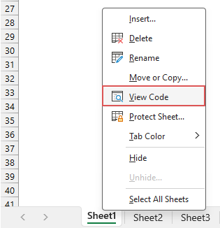
- คลิกขวาที่ชื่อแผ่นงานแล้วเลือก ดูรหัส จากเมนูบริบทดูภาพหน้าจอ:
- ในตัวแก้ไขโมดูลแผ่นงาน VBA ที่เปิดอยู่ ให้คัดลอกและวางโค้ดต่อไปนี้ลงในโมดูลเปล่า ดูภาพหน้าจอ:
รหัส VBA: ไฮไลต์แถวและคอลัมน์ของเซลล์ที่เลือกโดยอัตโนมัติPrivate Sub Worksheet_SelectionChange(ByVal Target As Range) 'Update by Extendoffice Dim rowRange As Range Dim colRange As Range Dim activeCell As Range Set activeCell = Target.Cells(1, 1) Set rowRange = Rows(activeCell.Row) Set colRange = Columns(activeCell.Column) Cells.Interior.ColorIndex = xlNone rowRange.Interior.Color = RGB(248, 150, 171) colRange.Interior.Color = RGB(173, 233, 249) End Subเคล็ดลับ: ปรับแต่งโค้ด- หากต้องการเปลี่ยนสีไฮไลต์ คุณเพียงแค่ต้องแก้ไขค่า RGB ในสคริปต์ต่อไปนี้:
rowRange.Interior.Color = RGB(248, 150, 171)
colRange.Interior.Color = RGB(173, 233, 249) - หากต้องการเน้นเฉพาะทั้งแถวของเซลล์ที่เลือก ให้ลบหรือใส่เครื่องหมายอะพอสทรอฟีไว้ด้านหน้าบรรทัดนี้:
colRange.Interior.Color = RGB(173, 233, 249) - หากต้องการเน้นเฉพาะทั้งคอลัมน์ของเซลล์ที่เลือก ให้ลบหรือใส่ความคิดเห็น (เพิ่มเครื่องหมายอะพอสทรอฟี่ที่ด้านหน้า) บรรทัดนี้:
rowRange.Interior.Color = RGB(248, 150, 171)

- หากต้องการเปลี่ยนสีไฮไลต์ คุณเพียงแค่ต้องแก้ไขค่า RGB ในสคริปต์ต่อไปนี้:
- จากนั้น ปิดหน้าต่างตัวแก้ไข VBA เพื่อกลับไปยังเวิร์กชีต
ผลลัพธ์:
ตอนนี้ เมื่อคุณเลือกเซลล์ ทั้งแถวและคอลัมน์ของเซลล์นั้นจะถูกไฮไลต์โดยอัตโนมัติ และไฮไลต์จะเปลี่ยนแบบไดนามิกเมื่อเซลล์ที่เลือกเปลี่ยนไปตามตัวอย่างด้านล่าง:
- รหัสนี้จะล้างสีพื้นหลังออกจากเซลล์ทั้งหมดในเวิร์กชีต ดังนั้น ให้หลีกเลี่ยงการใช้โซลูชันนี้หากคุณมีเซลล์ที่มีการระบายสีแบบกำหนดเอง
- การเรียกใช้รหัสนี้จะปิดการใช้งาน แก้ ในแผ่นงาน หมายความว่าคุณไม่สามารถย้อนกลับข้อผิดพลาดใดๆ ได้โดยการกดปุ่ม Ctrl + Z ทางลัด
- รหัสนี้จะไม่ทำงานในแผ่นงานที่มีการป้องกัน
- หากต้องการหยุดเน้นแถวและคอลัมน์ของเซลล์ที่เลือก คุณจะต้องลบโค้ด VBA ที่เพิ่มไว้ก่อนหน้านี้ หลังจากนั้นให้รีเซ็ตการไฮไลต์โดยคลิก หน้าแรก > เติมสี > ไม่มีการเติม.
เน้นแถวและคอลัมน์ที่ใช้งานอยู่โดยอัตโนมัติด้วยการคลิก Kutools เพียงคลิกเดียว
เผชิญกับข้อ จำกัด ของโค้ด VBA ใน Excel หรือไม่ Kutools สำหรับ Excel's กริดโฟกัส คุณลักษณะนี้เป็นทางออกที่ดีที่สุดของคุณ! ออกแบบมาเพื่อแก้ไขข้อบกพร่องของ VBA โดยนำเสนอสไตล์การไฮไลต์ที่หลากหลายเพื่อปรับปรุงประสบการณ์การใช้งานชีตของคุณ ด้วยความสามารถในการใช้สไตล์เหล่านี้กับสมุดงานที่เปิดอยู่ทั้งหมด Kutools ช่วยให้มั่นใจได้ถึงกระบวนการจัดการข้อมูลที่มีประสิทธิภาพและดึงดูดสายตาอย่างต่อเนื่อง
หลังจากการติดตั้ง Kutools สำหรับ Excelกรุณาคลิกที่ Kutools > กริดโฟกัส เพื่อเปิดใช้งานคุณสมบัตินี้ ตอนนี้คุณสามารถเห็นแถวและคอลัมน์ของเซลล์ที่ใช้งานอยู่ถูกเน้นทันที ไฮไลต์นี้จะเลื่อนไปตามแบบไดนามิกเมื่อคุณเปลี่ยนการเลือกเซลล์ ดูการสาธิตด้านล่าง:
- คงสีพื้นหลังของเซลล์ดั้งเดิมไว้:
ฟีเจอร์นี้ต่างจากโค้ด VBA โดยยึดตามการจัดรูปแบบที่มีอยู่ของเวิร์กชีตของคุณ - ใช้งานได้ในแผ่นป้องกัน:
คุณลักษณะนี้ทำงานได้อย่างราบรื่นภายในแผ่นงานที่ได้รับการป้องกัน ทำให้เหมาะสำหรับการจัดการเอกสารที่ละเอียดอ่อนหรือเอกสารที่แชร์โดยไม่กระทบต่อความปลอดภัย - ไม่ส่งผลกระทบต่อฟังก์ชัน Undo:
ด้วยคุณลักษณะนี้ คุณจะยังคงสามารถเข้าถึงฟังก์ชันการเลิกทำของ Excel ได้อย่างเต็มที่ สิ่งนี้ทำให้แน่ใจได้ว่าคุณสามารถคืนค่าการเปลี่ยนแปลงได้อย่างง่ายดาย โดยเพิ่มชั้นความปลอดภัยให้กับการจัดการข้อมูลของคุณ - ประสิทธิภาพที่เสถียรพร้อมข้อมูลขนาดใหญ่:
คุณสมบัตินี้ออกแบบมาเพื่อจัดการชุดข้อมูลขนาดใหญ่อย่างมีประสิทธิภาพ ทำให้มั่นใจได้ถึงประสิทธิภาพที่เสถียรแม้ในสเปรดชีตที่ซับซ้อนและมีข้อมูลจำนวนมาก - ไฮไลท์หลายสไตล์:
คุณลักษณะนี้นำเสนอตัวเลือกการไฮไลต์ที่หลากหลาย ช่วยให้คุณสามารถเลือกสไตล์และสีต่างๆ เพื่อทำให้เซลล์ของแถว คอลัมน์ หรือแถวและคอลัมน์ที่ใช้งานอยู่ของคุณโดดเด่นในลักษณะที่ตรงกับความต้องการและความต้องการของคุณมากที่สุด
- หากต้องการปิดใช้งานคุณลักษณะนี้ โปรดคลิก Kutools > กริดโฟกัส อีกครั้งเพื่อปิดฟังก์ชันนี้
- หากต้องการใช้คุณลักษณะนี้ โปรด ดาวน์โหลดและติดตั้ง Kutools สำหรับ Excel ก่อน
เน้นแถวและคอลัมน์ที่ใช้งานอยู่โดยอัตโนมัติด้วยการจัดรูปแบบตามเงื่อนไข
ใน Excel คุณยังสามารถตั้งค่าการจัดรูปแบบตามเงื่อนไขเพื่อเน้นแถวและคอลัมน์ที่ใช้งานอยู่โดยอัตโนมัติได้ สำหรับการตั้งค่าคุณสมบัตินี้ โปรดทำตามขั้นตอนเหล่านี้:
ขั้นตอนที่ 1: เลือกช่วงข้อมูล
ขั้นแรก เลือกช่วงของเซลล์ที่คุณต้องการใช้ฟีเจอร์นี้ นี่อาจเป็นทั้งเวิร์กชีตหรือชุดข้อมูลเฉพาะ ที่นี่ฉันจะเลือกทั้งแผ่นงาน
ขั้นตอนที่ 2: เข้าถึงการจัดรูปแบบตามเงื่อนไข
คลิก หน้าแรก > การจัดรูปแบบตามเงื่อนไข > กฎใหม่ดูภาพหน้าจอ:
ขั้นตอนที่ 3: ตั้งค่าการดำเนินการในกฎการจัดรูปแบบใหม่
- ตัว Vortex Indicator ได้ถูกนำเสนอลงในนิตยสาร กฎการจัดรูปแบบใหม่ ให้เลือก ใช้สูตรเพื่อกำหนดเซลล์ที่จะจัดรูปแบบ จาก เลือกประเภทกฎ กล่องรายการ
- ตัว Vortex Indicator ได้ถูกนำเสนอลงในนิตยสาร จัดรูปแบบค่าโดยที่สูตรนี้เป็นจริง ให้ป้อนสูตรใดสูตรหนึ่งต่อไปนี้ ในตัวอย่างนี้ ฉันจะใช้สูตรที่สามเพื่อเน้นแถวและคอลัมน์ที่ใช้งานอยู่
หากต้องการเน้นแถวที่ใช้งานอยู่:
หากต้องการเน้นคอลัมน์ที่ใช้งานอยู่:=CELL("row")=ROW()
หากต้องการเน้นแถวและคอลัมน์ที่ใช้งานอยู่:=CELL("col")=COLUMN()=OR(CELL("row")=ROW(), CELL("col")= COLUMN()) - จากนั้นคลิก รูปแบบ ปุ่ม

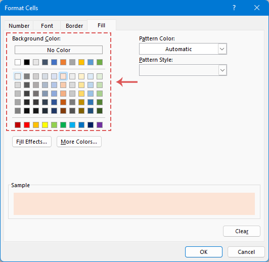
- ในเรื่องดังต่อไปนี้ จัดรูปแบบเซลล์ ภายใต้ ใส่ เลือกหนึ่งสีเพื่อเน้นแถวและคอลัมน์ที่ใช้งานอยู่ตามที่คุณต้องการ ดูภาพหน้าจอ:
- จากนั้นคลิก OK > OK เพื่อปิดกล่องโต้ตอบ
ผลลัพธ์:
ตอนนี้คุณสามารถเห็นทั้งคอลัมน์และแถวของเซลล์ A1 ได้รับการเน้นในครั้งเดียว หากต้องการใช้การไฮไลต์นี้กับเซลล์อื่น เพียงคลิกเซลล์ที่คุณต้องการแล้วกดปุ่ม F9 เพื่อรีเฟรชแผ่นงาน ซึ่งจะไฮไลต์ทั้งคอลัมน์และแถวของเซลล์ที่เลือกใหม่
- ที่จริงแล้ว แม้ว่าแนวทางการจัดรูปแบบตามเงื่อนไขสำหรับการเน้นใน Excel จะช่วยแก้ปัญหาได้ แต่ก็ไม่ได้ราบรื่นเหมือนการใช้งาน VBA และ กริดโฟกัส คุณสมบัติ. วิธีการนี้จำเป็นต้องคำนวณแผ่นงานใหม่ด้วยตนเอง (ทำได้โดยการกดปุ่ม F9 สำคัญ).
หากต้องการเปิดใช้งานการคำนวณใหม่โดยอัตโนมัติของเวิร์กชีทของคุณ คุณสามารถรวมโค้ด VBA แบบธรรมดาลงในโมดูลโค้ดของชีตเป้าหมายของคุณได้ การดำเนินการนี้จะทำให้กระบวนการรีเฟรชเป็นไปโดยอัตโนมัติ เพื่อให้แน่ใจว่าการไฮไลต์จะอัปเดตทันทีเมื่อคุณเลือกเซลล์อื่นโดยไม่ต้องกดปุ่ม F9 สำคัญ. โปรดคลิกขวาที่ชื่อแผ่นงาน จากนั้นเลือก ดูรหัส จากเมนูบริบท จากนั้นคัดลอกและวางโค้ดต่อไปนี้ลงในโมดูลชีต:Private Sub Worksheet_SelectionChange(ByVal Target As Range) Target.Calculate End Sub - การจัดรูปแบบตามเงื่อนไขจะรักษาการจัดรูปแบบที่มีอยู่ซึ่งคุณได้นำไปใช้กับเวิร์กชีตของคุณด้วยตนเอง
- การจัดรูปแบบตามเงื่อนไขเป็นที่รู้กันว่ามีความผันผวน โดยเฉพาะอย่างยิ่งเมื่อใช้กับชุดข้อมูลขนาดใหญ่มาก การใช้งานอย่างกว้างขวางอาจทำให้ประสิทธิภาพเวิร์กบุ๊กของคุณช้าลง ซึ่งส่งผลต่อประสิทธิภาพของการประมวลผลข้อมูลและการนำทาง
- ฟังก์ชัน CELL ใช้ได้เฉพาะใน Excel เวอร์ชัน 2007 และใหม่กว่า วิธีการนี้เข้ากันไม่ได้กับ Excel เวอร์ชันก่อนหน้า
การเปรียบเทียบวิธีการข้างต้น
| ลักษณะ | รหัส VBA | การจัดรูปแบบตามเงื่อนไข | Kutools สำหรับ Excel |
| รักษาสีพื้นหลังของเซลล์ | ไม่ | ใช่ | ใช่ |
| รองรับการเลิกทำ | ไม่ | ใช่ | ใช่ |
| มีเสถียรภาพในชุดข้อมูลขนาดใหญ่ | ไม่ | ไม่ | ใช่ |
| ใช้งานได้ในแผ่นป้องกัน | ไม่ | ใช่ | ใช่ |
| ใช้กับเวิร์กบุ๊กที่เปิดอยู่ทั้งหมด | เฉพาะแผ่นปัจจุบันเท่านั้น | เฉพาะแผ่นปัจจุบันเท่านั้น | สมุดงานที่เปิดอยู่ทั้งหมด |
| ต้องรีเฟรชด้วยตนเอง (F9) | ไม่ | ใช่ | ไม่ |
ซึ่งสรุปคำแนะนำของเราเกี่ยวกับวิธีเน้นคอลัมน์และแถวของเซลล์ที่เลือกใน Excel หากคุณสนใจที่จะสำรวจเคล็ดลับและลูกเล่น Excel เพิ่มเติม เว็บไซต์ของเรามีบทช่วยสอนหลายพันรายการ คลิกที่นี่เพื่อเข้าถึงพวกเขา. ขอขอบคุณที่อ่าน และเราหวังว่าจะให้ข้อมูลที่เป็นประโยชน์เพิ่มเติมแก่คุณในอนาคต!
บทความที่เกี่ยวข้อง:
- ไฮไลต์แถวและคอลัมน์ของเซลล์ที่ใช้งานอยู่โดยอัตโนมัติ
- เมื่อคุณดูเวิร์กชีตขนาดใหญ่ที่มีข้อมูลจำนวนมากคุณอาจต้องการเน้นแถวและคอลัมน์ของเซลล์ที่เลือกเพื่อให้คุณสามารถอ่านข้อมูลได้อย่างง่ายดายและโดยสังหรณ์ใจเพื่อหลีกเลี่ยงการอ่านผิด ที่นี่ฉันสามารถแนะนำเคล็ดลับที่น่าสนใจเพื่อเน้นแถวและคอลัมน์ของเซลล์ปัจจุบันเมื่อเซลล์เปลี่ยนไปคอลัมน์และแถวของเซลล์ใหม่จะถูกไฮไลต์โดยอัตโนมัติ
- เน้นแถวหรือคอลัมน์อื่นๆ ทุกแถวใน Excel
- ในเวิร์กชีตขนาดใหญ่ การเน้นหรือการเติมแถวหรือคอลัมน์ที่ n หรืออื่นๆ จะช่วยเพิ่มการมองเห็นข้อมูลและความสามารถในการอ่าน ไม่เพียงแต่ทำให้เวิร์กชีตดูเรียบร้อยขึ้นเท่านั้น แต่ยังช่วยให้คุณเข้าใจข้อมูลได้เร็วขึ้นอีกด้วย ในบทความนี้ เราจะแนะนำวิธีการต่างๆ เพื่อแรเงาแถวหรือคอลัมน์อื่นๆ หรือแถวที่ n ซึ่งช่วยให้คุณนำเสนอข้อมูลในลักษณะที่น่าสนใจและตรงไปตรงมามากขึ้น
- ไฮไลต์ทั้งแถว/ทั้งแถวขณะเลื่อน
- หากคุณมีแผ่นงานขนาดใหญ่ที่มีหลายคอลัมน์คุณจะแยกแยะข้อมูลในแถวนั้นได้ยาก ในกรณีนี้คุณสามารถเน้นทั้งแถวของเซลล์ที่ใช้งานอยู่เพื่อให้คุณสามารถดูข้อมูลในแถวนั้นได้อย่างรวดเร็วและง่ายดายเมื่อคุณเลื่อนแถบเลื่อนแนวนอนลงบทความนี้ฉันจะพูดถึงเทคนิคบางอย่างสำหรับคุณในการแก้ปัญหานี้ .
- ไฮไลต์แถวตามรายการแบบเลื่อนลง
- บทความนี้จะพูดถึงวิธีการเน้นแถวตามรายการแบบเลื่อนลงใช้ภาพหน้าจอต่อไปนี้เช่นเมื่อฉันเลือก“ กำลังดำเนินการ” จากรายการแบบเลื่อนลงในคอลัมน์ E ฉันต้องเน้นแถวนี้ด้วยสีแดงเมื่อฉัน เลือก "เสร็จสมบูรณ์" จากรายการแบบเลื่อนลงฉันต้องเน้นแถวนี้ด้วยสีน้ำเงินและเมื่อฉันเลือก "ยังไม่เริ่ม" ระบบจะใช้สีเขียวเพื่อเน้นแถว
สุดยอดเครื่องมือเพิ่มผลผลิตในสำนักงาน
เพิ่มพูนทักษะ Excel ของคุณด้วย Kutools สำหรับ Excel และสัมผัสประสิทธิภาพอย่างที่ไม่เคยมีมาก่อน Kutools สำหรับ Excel เสนอคุณสมบัติขั้นสูงมากกว่า 300 รายการเพื่อเพิ่มประสิทธิภาพและประหยัดเวลา คลิกที่นี่เพื่อรับคุณสมบัติที่คุณต้องการมากที่สุด...
")
แท็บ Office นำอินเทอร์เฟซแบบแท็บมาที่ Office และทำให้งานของคุณง่ายขึ้นมาก
- เปิดใช้งานการแก้ไขและอ่านแบบแท็บใน Word, Excel, PowerPoint, ผู้จัดพิมพ์, Access, Visio และโครงการ
- เปิดและสร้างเอกสารหลายรายการในแท็บใหม่ของหน้าต่างเดียวกันแทนที่จะเป็นในหน้าต่างใหม่
- เพิ่มประสิทธิภาพการทำงานของคุณ 50% และลดการคลิกเมาส์หลายร้อยครั้งให้คุณทุกวัน!
")