จะเปลี่ยนตัวเลขเชิงลบเป็นบวกใน Excel ได้อย่างไร?
เมื่อคุณกำลังประมวลผลการดำเนินการใน Excel บางครั้งคุณอาจต้องเปลี่ยนตัวเลขเชิงลบเป็นตัวเลขบวกหรือในทางกลับกัน มีกลเม็ดง่ายๆที่คุณสามารถใช้เพื่อเปลี่ยนจำนวนลบเป็นบวกได้หรือไม่? บทความนี้จะแนะนำเคล็ดลับต่อไปนี้สำหรับการแปลงจำนวนลบทั้งหมดให้เป็นบวกหรือในทางกลับกันอย่างง่ายดาย
เปลี่ยนจำนวนลบเป็นบวกด้วยฟังก์ชันพิเศษวาง
เปลี่ยนตัวเลขเชิงลบเป็นบวกได้อย่างง่ายดายด้วย Kutools for Excel
เปลี่ยนจำนวนลบเป็นบวกด้วยฟังก์ชันพิเศษวาง

คุณสามารถเปลี่ยนจำนวนลบเป็นจำนวนบวกได้โดยทำตามขั้นตอนต่อไปนี้:
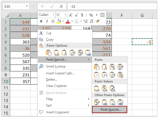
1. ป้อนหมายเลข -1 ในเซลล์ว่างจากนั้นเลือกเซลล์นี้แล้วกด Ctrl + C คีย์เพื่อคัดลอก
2. เลือกจำนวนลบทั้งหมดในช่วงนั้นคลิกขวาแล้วเลือก วางพิเศษ ... จากเมนูบริบท ดูภาพหน้าจอ:
(1) การถือครอง Ctrl คุณสามารถเลือกตัวเลขเชิงลบทั้งหมดโดยคลิกทีละตัว
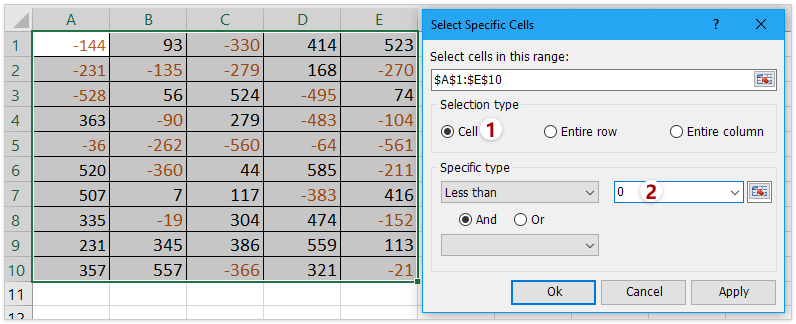
(2) หากคุณติดตั้ง Kutools for Excel ไว้คุณสามารถใช้ไฟล์ เลือกเซลล์พิเศษ คุณสมบัติในการเลือกจำนวนลบทั้งหมดอย่างรวดเร็ว ทดลองใช้ฟรี!
3. และ a วางแบบพิเศษ กล่องโต้ตอบจะปรากฏขึ้นให้เลือก ทั้งหมด ตัวเลือกจาก พาสต้าให้เลือก คูณ ตัวเลือกจาก การดำเนินการคลิก OK. ดูภาพหน้าจอ:

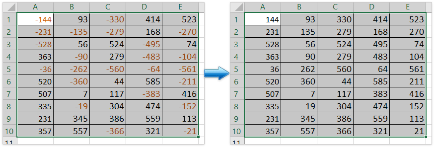
4. จำนวนลบที่เลือกทั้งหมดจะถูกแปลงเป็นจำนวนบวก ลบหมายเลข -1 ตามที่คุณต้องการ ดูภาพหน้าจอ:

เปลี่ยนตัวเลขเชิงลบเป็นบวกได้อย่างง่ายดายในช่วงที่ระบุใน Excel
เมื่อเปรียบเทียบกับการลบเครื่องหมายลบออกจากเซลล์ทีละเซลล์ด้วยตนเอง Kutools for Excel's เปลี่ยนสัญลักษณ์ของค่า คุณลักษณะนี้เป็นวิธีที่ง่ายมากในการเปลี่ยนตัวเลขเชิงลบทั้งหมดเป็นค่าบวกในการเลือกอย่างรวดเร็ว ทดลองใช้ฟีเจอร์เต็มรูปแบบฟรี 30 วันทันที!
Kutools สำหรับ Excel - เพิ่มประสิทธิภาพ Excel ด้วยเครื่องมือที่จำเป็นมากกว่า 300 รายการ เพลิดเพลินกับฟีเจอร์ทดลองใช้ฟรี 30 วันโดยไม่ต้องใช้บัตรเครดิต! Get It Now
เปลี่ยนตัวเลขเชิงลบให้เป็นบวกได้อย่างรวดเร็วและง่ายดายด้วย Kutools for Excel
ผู้ใช้ Excel ส่วนใหญ่ไม่ต้องการใช้โค้ด VBA มีเคล็ดลับง่ายๆในการเปลี่ยนตัวเลขเชิงลบเป็นบวกหรือไม่? Kutools สำหรับ excel สามารถช่วยให้คุณบรรลุเป้าหมายนี้ได้อย่างง่ายดายและสะดวกสบาย
Kutools สำหรับ Excel - เพิ่มประสิทธิภาพ Excel ด้วยเครื่องมือที่จำเป็นมากกว่า 300 รายการ เพลิดเพลินกับฟีเจอร์ทดลองใช้ฟรี 30 วันโดยไม่ต้องใช้บัตรเครดิต! Get It Now
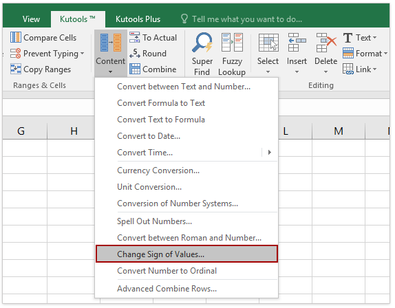
1. เลือกช่วงซึ่งรวมถึงตัวเลขเชิงลบที่คุณต้องการเปลี่ยนแล้วคลิก Kutools > คอนเทนต์ > เปลี่ยนสัญลักษณ์ของค่า.
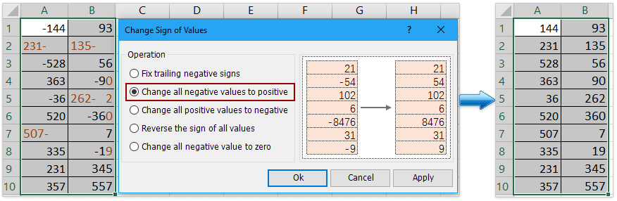
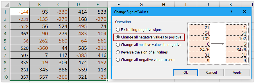
2. การตรวจสอบ เปลี่ยนค่าลบทั้งหมดเป็นค่าบวก ภายใต้ การดำเนินการและคลิก Ok. ดูภาพหน้าจอ:
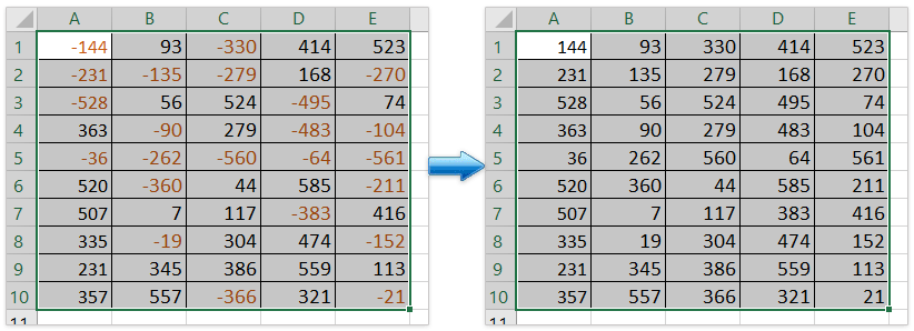
ตอนนี้คุณจะเห็นตัวเลขเชิงลบทั้งหมดเปลี่ยนเป็นตัวเลขบวกดังที่แสดงด้านล่าง:
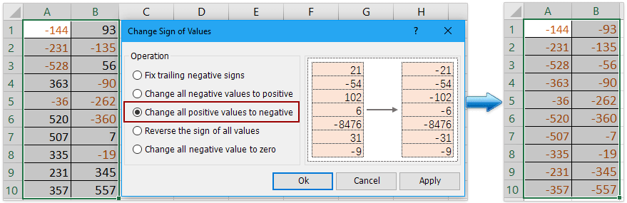
หมายเหตุ: ด้วยสิ่งนี้ เปลี่ยนสัญลักษณ์ของค่า คุณยังสามารถแก้ไขเครื่องหมายลบต่อท้ายเปลี่ยนตัวเลขบวกทั้งหมดเป็นลบย้อนกลับเครื่องหมายของค่าทั้งหมดและเปลี่ยนค่าลบทั้งหมดเป็นศูนย์ ทดลองใช้ฟรี!
(1) เปลี่ยนค่าบวกทั้งหมดเป็นค่าลบอย่างรวดเร็วในช่วงที่ระบุ:
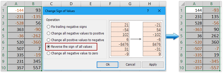
(2) ย้อนกลับสัญลักษณ์ของค่าทั้งหมดในช่วงที่ระบุได้อย่างง่ายดาย:
(3) เปลี่ยนค่าลบทั้งหมดเป็นศูนย์ในช่วงที่ระบุได้อย่างง่ายดาย:

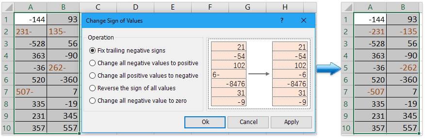
(4) แก้ไขเครื่องหมายเชิงลบต่อท้ายในช่วงที่ระบุได้อย่างง่ายดาย:
ใช้รหัส VBA เพื่อแปลงจำนวนลบทั้งหมดของช่วงเป็นบวก
ในฐานะผู้เชี่ยวชาญของ Excel คุณสามารถเรียกใช้รหัส VBA เพื่อเปลี่ยนตัวเลขเชิงลบเป็นตัวเลขบวกได้
1. กด Alt + F11 เพื่อเปิดหน้าต่าง Microsoft Visual Basic for Applications
2. จะมีหน้าต่างใหม่ปรากฏขึ้น คลิก สิ่งที่ใส่เข้าไป > โมดูลจากนั้นป้อนรหัสต่อไปนี้ในโมดูล:
Sub Positive
Dim Cel As Range
For Each Cel In Selection
If IsNumeric(Cel.Value) Then
Cel.Value = Abs(Cel.Value)
End If
Next Cel
End Sub3. จากนั้นคลิก วิ่ง หรือกด F5 คีย์เพื่อเรียกใช้แอปพลิเคชันและตัวเลขเชิงลบทั้งหมดจะเปลี่ยนเป็นตัวเลขบวก ดูภาพหน้าจอ:
การสาธิต: เปลี่ยนตัวเลขเชิงลบเป็นบวกหรือในทางกลับกันด้วย Kutools for Excel
บทความที่เกี่ยวข้อง
ย้อนกลับสัญญาณของค่าในเซลล์
เมื่อเราใช้ excel มีทั้งตัวเลขบวกและลบในแผ่นงาน สมมติว่าเราจำเป็นต้องเปลี่ยนจำนวนบวกเป็นลบและในทางกลับกัน แน่นอนว่าเราสามารถเปลี่ยนได้ด้วยตนเอง แต่หากต้องเปลี่ยนตัวเลขหลายร้อยตัววิธีนี้ก็ไม่ใช่ทางเลือกที่ดี มีเคล็ดลับง่ายๆในการแก้ปัญหานี้หรือไม่?
เปลี่ยนจำนวนบวกเป็นลบ
คุณจะเปลี่ยนตัวเลขหรือค่าบวกทั้งหมดเป็นค่าลบใน Excel ได้อย่างไร? วิธีการต่อไปนี้สามารถแนะนำให้คุณเปลี่ยนตัวเลขบวกทั้งหมดเป็นลบใน Excel ได้อย่างรวดเร็ว
แก้ไขสัญญาณลบต่อท้ายในเซลล์
ด้วยเหตุผลบางประการคุณอาจต้องแก้ไขเครื่องหมายลบต่อท้ายในเซลล์ใน Excel ตัวอย่างเช่นตัวเลขที่มีเครื่องหมายลบต่อท้ายจะเป็น 90- ในสภาพนี้คุณจะแก้ไขเครื่องหมายลบต่อท้ายได้อย่างไรโดยการลบเครื่องหมายลบต่อท้ายจากขวาไปซ้าย นี่คือกลเม็ดง่ายๆที่สามารถช่วยคุณได้
เปลี่ยนจำนวนลบเป็นศูนย์
ฉันจะแนะนำให้คุณเปลี่ยนตัวเลขลบทั้งหมดให้เป็นศูนย์พร้อมกันในส่วนที่เลือก
เครื่องมือเพิ่มประสิทธิภาพการทำงานในสำนักงานที่ดีที่สุด
Kutools สำหรับ Excel - ช่วยให้คุณโดดเด่นจากฝูงชน
Kutools สำหรับ Excel มีคุณสมบัติมากกว่า 300 รายการ รับรองว่าสิ่งที่คุณต้องการเพียงแค่คลิกเดียว...
")
แท็บ Office - เปิดใช้งานการอ่านแบบแท็บและการแก้ไขใน Microsoft Office (รวม Excel)
- หนึ่งวินาทีเพื่อสลับไปมาระหว่างเอกสารที่เปิดอยู่มากมาย!
- ลดการคลิกเมาส์หลายร้อยครั้งสำหรับคุณทุกวันบอกลามือเมาส์
- เพิ่มประสิทธิภาพการทำงานของคุณได้ถึง 50% เมื่อดูและแก้ไขเอกสารหลายฉบับ
- นำแท็บที่มีประสิทธิภาพมาสู่ Office (รวมถึง Excel) เช่นเดียวกับ Chrome, Edge และ Firefox
")