วิธีการเน้นเซลล์หรือแถวด้วยช่องทำเครื่องหมายใน Excel
ตามภาพหน้าจอด้านล่างคุณจะต้องเน้นแถวหรือเซลล์ด้วยช่องทำเครื่องหมาย เมื่อเลือกช่องทำเครื่องหมายแถวที่ระบุหรือเซลล์จะถูกไฮไลต์โดยอัตโนมัติ แต่จะบรรลุใน Excel ได้อย่างไร? บทความนี้จะแสดงสองวิธีในการบรรลุเป้าหมาย

ไฮไลต์เซลล์หรือแถวด้วยช่องทำเครื่องหมายด้วยการจัดรูปแบบตามเงื่อนไข
ไฮไลต์เซลล์หรือแถวด้วยช่องทำเครื่องหมายพร้อมรหัส VBA
ไฮไลต์เซลล์หรือแถวด้วยช่องทำเครื่องหมายด้วยการจัดรูปแบบตามเงื่อนไข
คุณสามารถสร้างกฎการจัดรูปแบบตามเงื่อนไขเพื่อเน้นเซลล์หรือแถวด้วยช่องทำเครื่องหมายใน Excel กรุณาดำเนินการดังนี้
เชื่อมโยงกล่องกาเครื่องหมายทั้งหมดกับเซลล์ที่ระบุ
1. คุณต้องแทรกช่องทำเครื่องหมายลงในเซลล์ทีละเซลล์ด้วยตนเองโดยคลิก ผู้พัฒนา > สิ่งที่ใส่เข้าไป > ทำเครื่องหมายในช่อง (การควบคุมแบบฟอร์ม).
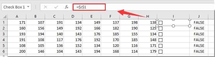
2. ตอนนี้กล่องกาเครื่องหมายถูกแทรกลงในเซลล์ในคอลัมน์ I แล้วโปรดเลือกกล่องกาเครื่องหมายแรกใน I1 ป้อนสูตร = $ J1 ลงในแถบสูตรแล้วกด เข้าสู่ กุญแจ
ปลาย: ถ้าคุณไม่ต้องการให้มีค่าที่เชื่อมโยงกับเซลล์ที่อยู่ติดกันกับช่องทำเครื่องหมายคุณสามารถเชื่อมโยงช่องทำเครื่องหมายกับเซลล์ของแผ่นงานอื่นเช่น = Sheet3! $ E1.
2. ทำซ้ำขั้นตอนที่ 1 จนกว่ากล่องกาเครื่องหมายทั้งหมดจะเชื่อมโยงกับเซลล์หรือเซลล์ที่อยู่ติดกันในแผ่นงานอื่น
หมายเหตุ: เซลล์ที่เชื่อมโยงทั้งหมดควรอยู่ต่อเนื่องกันและอยู่ในคอลัมน์เดียวกัน
สร้างกฎการจัดรูปแบบตามเงื่อนไข
ตอนนี้คุณต้องสร้างกฎการจัดรูปแบบตามเงื่อนไขตามขั้นตอนต่อไปนี้
1. เลือกแถวที่คุณต้องการเน้นด้วยช่องทำเครื่องหมายจากนั้นคลิก การจัดรูปแบบตามเงื่อนไข > กฎใหม่ ภายใต้ หน้าแรก แท็บ ดูภาพหน้าจอ:

2 ใน กฎการจัดรูปแบบใหม่ คุณต้อง:
2.1 เลือกไฟล์ ใช้สูตรเพื่อกำหนดเซลล์ที่จะจัดรูปแบบ ตัวเลือกใน เลือกประเภทกฎ กล่อง;
2.2 ป้อนสูตร = IF ($ J1 = จริงจริงเท็จ) เข้าไปใน จัดรูปแบบค่าโดยที่สูตรนี้เป็นจริง กล่อง;
Or = IF (Sheet3! $ E1 = TRUE, TRUE, FALSE) ถ้ากล่องกาเครื่องหมายเชื่อมโยงกับแผ่นงานอื่น
2.3 คลิกปุ่ม รูปแบบ ปุ่มเพื่อระบุสีที่ไฮไลต์สำหรับแถว
2.4 คลิกปุ่ม OK ปุ่ม. ดูภาพหน้าจอ:

หมายเหตุ: ในสูตร $ J1 or $ E1 เป็นเซลล์แรกที่เชื่อมโยงสำหรับกล่องกาเครื่องหมายและตรวจสอบให้แน่ใจว่าการอ้างอิงเซลล์ถูกเปลี่ยนเป็นคอลัมน์สัมบูรณ์ (J1> $ J1 or E1> $ E1).
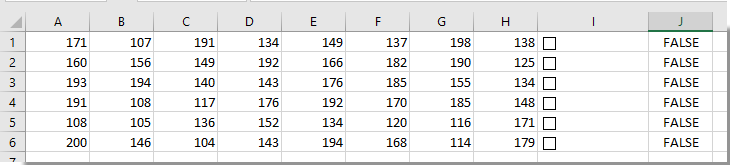
ตอนนี้กฎการจัดรูปแบบตามเงื่อนไขถูกสร้างขึ้น เมื่อเลือกช่องทำเครื่องหมายแถวที่เกี่ยวข้องจะถูกไฮไลต์โดยอัตโนมัติเมื่อแสดงภาพหน้าจอของเครื่องสูบลม

ไฮไลต์เซลล์หรือแถวด้วยช่องทำเครื่องหมายพร้อมรหัส VBA
รหัส VBA ต่อไปนี้สามารถช่วยคุณในการเน้นเซลล์หรือแถวด้วยช่องทำเครื่องหมายใน Excel กรุณาดำเนินการดังนี้
1. ในแผ่นงานคุณต้องเน้นเซลล์หรือแถวด้วยช่องทำเครื่องหมาย คลิกขวาที่ไฟล์ แท็บแผ่นงาน และเลือก ดูรหัส จากเมนูคลิกขวาเพื่อเปิดไฟล์ Microsoft Visual Basic สำหรับแอปพลิเคชัน หน้าต่าง
2. จากนั้นคัดลอกและวางโค้ด VBA ด้านล่างลงในหน้าต่างรหัส
รหัส VBA: เน้นแถวที่มีช่องทำเครื่องหมายใน Excel
Sub AddCheckBox()
Dim xCell As Range
Dim xRng As Range
Dim I As Integer
Dim xChk As CheckBox
On Error Resume Next
InputC:
    Set xRng = Application.InputBox("Please select the column range to insert checkboxes:", "Kutools for Excel", Selection.Address, , , , , 8)
If xRng Is Nothing Then Exit Sub
If xRng.Columns.Count > 1 Then
    MsgBox "The selected range should be a single column", vbInformation, "Kutools fro Excel"
    GoTo InputC
Else
    If xRng.Columns.Count = 1 Then
        For Each xCell In xRng
            With ActiveSheet.CheckBoxes.Add(xCell.Left, _
               xCell.Top, xCell.Width = 15, xCell.Height = 12)
               .LinkedCell = xCell.Offset(, 1).Address(External:=False)
               .Interior.ColorIndex = xlNone
               .Caption = ""
               .Name = "Check Box " & xCell.Row
            End With
            xRng.Rows(xCell.Row).Interior.ColorIndex = xlNone
        Next
    End If
    With xRng
     .Rows.RowHeight = 16
    End With
    xRng.ColumnWidth = 5#
    xRng.Cells(1, 1).Offset(0, 1).Select
    For Each xChk In ActiveSheet.CheckBoxes
      xChk.OnAction = ActiveSheet.Name + ".InsertBgColor"
    Next
End If
End Sub

Sub InsertBgColor()
Dim xName As Integer
Dim xChk As CheckBox
For Each xChk In ActiveSheet.CheckBoxes
  xName = Right(xChk.Name, Len(xChk.Name) - 10)
  If (xName = Range(xChk.LinkedCell).Row) Then
   If (Range(xChk.LinkedCell) = "True") Then
    Range("A" & xName, Range(xChk.LinkedCell).Offset(0, -2)).Interior.ColorIndex = 6
   Else
    Range("A" & xName, Range(xChk.LinkedCell).Offset(0, -2)).Interior.ColorIndex = xlNone
   End If
  End If
Next
End Sub
3 กด F5 กุญแจสำคัญในการเรียกใช้รหัส (หมายเหตุ: คุณควรวางเคอร์เซอร์ไว้ในส่วนแรกของรหัสเพื่อใช้ปุ่ม F5) ในป๊อปอัป Kutools สำหรับ Excel โปรดเลือกช่วงที่คุณต้องการแทรกกล่องกาเครื่องหมายจากนั้นคลิกที่ OK ปุ่ม. ที่นี่ฉันเลือกช่วง I1: I6 ดูภาพหน้าจอ:

4. จากนั้นใส่กล่องกาเครื่องหมายลงในเซลล์ที่เลือก เลือกช่องทำเครื่องหมายใด ๆ แถวที่เกี่ยวข้องจะถูกไฮไลต์โดยอัตโนมัติตามภาพด้านล่างที่แสดง

บทความที่เกี่ยวข้อง:
- วิธีเปลี่ยนค่าหรือสีของเซลล์ที่ระบุเมื่อเลือกช่องทำเครื่องหมายใน Excel
- จะแทรกการประทับวันที่ลงในเซลล์ได้อย่างไรหากเลือกช่องทำเครื่องหมายใน Excel
- จะตรวจสอบช่องทำเครื่องหมายตามค่าเซลล์ใน Excel ได้อย่างไร
- วิธีกรองข้อมูลตามช่องทำเครื่องหมายใน Excel
- วิธีซ่อนช่องทำเครื่องหมายเมื่อซ่อนแถวใน Excel
- วิธีสร้างรายการแบบหล่นลงพร้อมช่องทำเครื่องหมายหลายช่องใน Excel
สุดยอดเครื่องมือเพิ่มผลผลิตในสำนักงาน
เพิ่มพูนทักษะ Excel ของคุณด้วย Kutools สำหรับ Excel และสัมผัสประสิทธิภาพอย่างที่ไม่เคยมีมาก่อน Kutools สำหรับ Excel เสนอคุณสมบัติขั้นสูงมากกว่า 300 รายการเพื่อเพิ่มประสิทธิภาพและประหยัดเวลา คลิกที่นี่เพื่อรับคุณสมบัติที่คุณต้องการมากที่สุด...
")
แท็บ Office นำอินเทอร์เฟซแบบแท็บมาที่ Office และทำให้งานของคุณง่ายขึ้นมาก
- เปิดใช้งานการแก้ไขและอ่านแบบแท็บใน Word, Excel, PowerPoint, ผู้จัดพิมพ์, Access, Visio และโครงการ
- เปิดและสร้างเอกสารหลายรายการในแท็บใหม่ของหน้าต่างเดียวกันแทนที่จะเป็นในหน้าต่างใหม่
- เพิ่มประสิทธิภาพการทำงานของคุณ 50% และลดการคลิกเมาส์หลายร้อยครั้งให้คุณทุกวัน!
")