ไปยังเนื้อหาหลัก

วิธีค้นหาค่าสูงสุดและส่งคืนค่าเซลล์ที่อยู่ติดกันใน Excel

doc-get-maximum-related-value-1 1

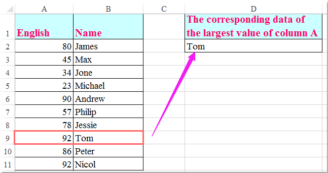
หากคุณมีช่วงข้อมูลดังภาพหน้าจอต่อไปนี้ตอนนี้คุณต้องการค้นหาค่าที่ใหญ่ที่สุดในคอลัมน์ A และรับเนื้อหาเซลล์ที่อยู่ติดกันในคอลัมน์ B ใน Excel คุณสามารถจัดการกับปัญหานี้ด้วยสูตรบางสูตรได้

ค้นหาค่าสูงสุดและส่งคืนค่าเซลล์ที่อยู่ติดกันด้วยสูตร

ค้นหาและเลือกค่าสูงสุดและส่งคืนค่าเซลล์ที่อยู่ติดกันด้วย Kutools for Excel


ลูกศรสีฟ้าฟองขวา ค้นหาค่าสูงสุดและส่งคืนค่าเซลล์ที่อยู่ติดกันด้วยสูตร

ใช้ข้อมูลข้างต้นเพื่อให้ได้ค่าที่มากที่สุดของข้อมูลที่เกี่ยวข้องคุณสามารถใช้สูตรต่อไปนี้:

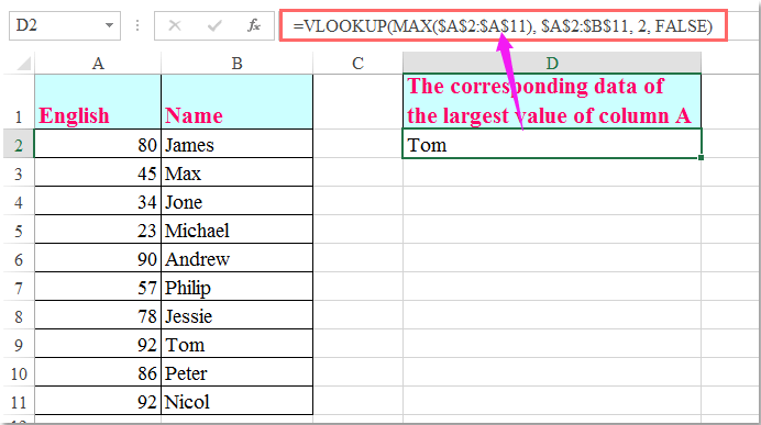
กรุณาพิมพ์สูตรนี้: = VLOOKUP (สูงสุด ($ A $ 2: $ A $ 11), $ A $ 2: $ B $ 11, 2, FALSE) ลงในเซลล์ว่างที่คุณต้องการจากนั้นกด เข้าสู่ คีย์เพื่อส่งคืนผลลัพธ์ที่ถูกต้องดูภาพหน้าจอ:

doc-get-maximum-related-value-2 2

หมายเหตุ:

1. ในสูตรข้างต้น A2: A11 คือช่วงข้อมูลที่คุณต้องการทราบค่าที่มากที่สุดและ A2: B11 ระบุช่วงข้อมูลที่คุณใช้จำนวน 2 คือหมายเลขคอลัมน์ที่ส่งคืนค่าที่ตรงกันของคุณ

2. หากมีค่าที่ใหญ่ที่สุดหลายค่าในคอลัมน์ A สูตรนี้จะได้รับค่าแรกเท่านั้น

3. ด้วยค่าด้านบนคุณสามารถส่งคืนค่าเซลล์จากคอลัมน์ด้านขวาหากคุณต้องการส่งคืนค่าที่อยู่ในคอลัมน์ด้านซ้ายคุณควรใช้สูตรนี้: =INDEX(A2:A11,MATCH(MAX(B2:B11),B2:B11,0))( A2: A11 คือช่วงข้อมูลที่คุณต้องการรับค่าสัมพัทธ์ B2: B11 คือช่วงข้อมูลที่มีค่ามากที่สุด) จากนั้นกด เข้าสู่ สำคัญ. คุณจะได้รับผลลัพธ์ดังต่อไปนี้:

doc-get-maximum-related-value-3 3


ลูกศรสีฟ้าฟองขวา ค้นหาและเลือกค่าสูงสุดและส่งคืนค่าเซลล์ที่อยู่ติดกันด้วย Kutools for Excel

สูตรข้างต้นสามารถช่วยให้คุณส่งคืนข้อมูลแรกที่เกี่ยวข้องเท่านั้นหากมีจำนวนมากที่สุดที่ซ้ำกันจะไม่ช่วย Kutools สำหรับ Excel's เลือกเซลล์ที่มีค่าสูงสุด & ต่ำสุด ยูทิลิตี้อาจช่วยให้คุณเลือกหมายเลขที่ใหญ่ที่สุดทั้งหมดจากนั้นคุณสามารถดูข้อมูลที่เกี่ยวข้องได้อย่างง่ายดายซึ่งเป็นส่วนเสริมของหมายเลขที่ใหญ่ที่สุด

หลังจากการติดตั้ง Kutools สำหรับ Excelโปรดดำเนินการดังนี้:

Kutools สำหรับ Excel : ด้วย Add-in ของ Excel ที่มีประโยชน์มากกว่า 300 รายการทดลองใช้ฟรีโดยไม่มีข้อ จำกัด ใน 30 วัน. 

1. เลือกคอลัมน์ตัวเลขที่คุณต้องการค้นหาและเลือกค่าที่มากที่สุด

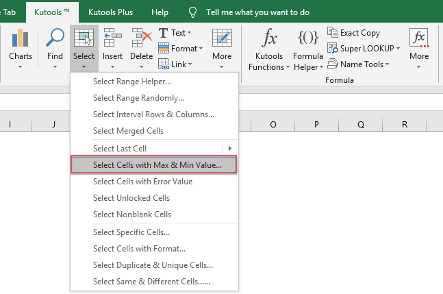
2. จากนั้นคลิก Kutools > เลือก > เลือกเซลล์ที่มีค่าสูงสุด & ต่ำสุดดูภาพหน้าจอ:

3. ใน เลือกเซลล์ที่มีค่าสูงสุด & ต่ำสุด ให้เลือก ค่าสูงสุด จาก ไปที่ ส่วนและเลือก เซลล์ ตัวเลือกใน ฐาน จากนั้นเลือก เซลล์ทั้งหมด or เซลล์แรกเท่านั้น ที่คุณต้องการเลือกค่ามากที่สุดให้คลิก OKจำนวนที่มากที่สุดในคอลัมน์ A ได้ถูกเลือกแล้วคุณจะได้รับข้อมูลที่เกี่ยวข้องซึ่งจะเพิ่มเข้าไปดูภาพหน้าจอ:

doc-get-maximum-related-value-5 5 2 doc-get-maximum-related-value-6 6

คลิกเพื่อดาวน์โหลด Kutools สำหรับ Excel และทดลองใช้ฟรีทันที!


บทความที่เกี่ยวข้อง:

วิธีค้นหาค่าสูงสุดในแถวและส่งคืนส่วนหัวของคอลัมน์ใน Excel

สุดยอดเครื่องมือเพิ่มผลผลิตในสำนักงาน

🤖 Kutools AI ผู้ช่วย: ปฏิวัติการวิเคราะห์ข้อมูลโดยยึดตาม: การดำเนินการที่ชาญฉลาด   |  สร้างรหัส  |  สร้างสูตรที่กำหนดเอง  |  วิเคราะห์ข้อมูลและสร้างแผนภูมิ  |  เรียกใช้ฟังก์ชัน Kutools...
คุณสมบัติยอดนิยม: ค้นหา เน้น หรือระบุรายการที่ซ้ำกัน   |  ลบแถวว่าง   |  รวมคอลัมน์หรือเซลล์โดยไม่สูญเสียข้อมูล   |   รอบโดยไม่มีสูตร ...
การค้นหาขั้นสูง: VLookup หลายเกณฑ์    VLookup หลายค่า  |   VLookup ข้ามหลายแผ่น   |   การค้นหาที่ไม่ชัดเจน ....
รายการแบบเลื่อนลงขั้นสูง: สร้างรายการแบบหล่นลงอย่างรวดเร็ว   |  รายการแบบหล่นลงขึ้นอยู่กับ   |  เลือกหลายรายการแบบหล่นลง ....
ผู้จัดการคอลัมน์: เพิ่มจำนวนคอลัมน์เฉพาะ  |  ย้ายคอลัมน์  |  สลับสถานะการมองเห็นของคอลัมน์ที่ซ่อนอยู่  |  เปรียบเทียบช่วงและคอลัมน์ ...
คุณสมบัติเด่น: กริดโฟกัส   |  มุมมองการออกแบบ   |   บาร์สูตรใหญ่    สมุดงานและตัวจัดการชีต   |  ห้องสมุดทรัพยากร (ข้อความอัตโนมัติ)   |  เลือกวันที่   |  รวมแผ่นงาน   |  เข้ารหัส/ถอดรหัสเซลล์    ส่งอีเมลตามรายการ   |  ซุปเปอร์ฟิลเตอร์   |   ตัวกรองพิเศษ (กรองตัวหนา/ตัวเอียง/ขีดทับ...) ...
ชุดเครื่องมือ 15 อันดับแรก12 ข้อความ เครื่องมือ (เพิ่มข้อความ, ลบอักขระ, ... )   |   50 + แผนภูมิ ประเภท (แผนภูมิ Gantt, ... )   |   40+ ใช้งานได้จริง สูตร (คำนวณอายุตามวันเกิด, ... )   |   19 การแทรก เครื่องมือ (ใส่ QR Code, แทรกรูปภาพจากเส้นทาง, ... )   |   12 การแปลง เครื่องมือ (ตัวเลขเป็นคำ, การแปลงสกุลเงิน, ... )   |   7 ผสานและแยก เครื่องมือ (แถวรวมขั้นสูง, แยกเซลล์, ... )   |   ... และอื่น ๆ

เพิ่มพูนทักษะ Excel ของคุณด้วย Kutools สำหรับ Excel และสัมผัสประสิทธิภาพอย่างที่ไม่เคยมีมาก่อน Kutools สำหรับ Excel เสนอคุณสมบัติขั้นสูงมากกว่า 300 รายการเพื่อเพิ่มประสิทธิภาพและประหยัดเวลา  คลิกที่นี่เพื่อรับคุณสมบัติที่คุณต้องการมากที่สุด...

รายละเอียด


แท็บ Office นำอินเทอร์เฟซแบบแท็บมาที่ Office และทำให้งานของคุณง่ายขึ้นมาก

  • เปิดใช้งานการแก้ไขและอ่านแบบแท็บใน Word, Excel, PowerPoint, ผู้จัดพิมพ์, Access, Visio และโครงการ
  • เปิดและสร้างเอกสารหลายรายการในแท็บใหม่ของหน้าต่างเดียวกันแทนที่จะเป็นในหน้าต่างใหม่
  • เพิ่มประสิทธิภาพการทำงานของคุณ 50% และลดการคลิกเมาส์หลายร้อยครั้งให้คุณทุกวัน!
Comments (13)
No ratings yet. Be the first to rate!
This comment was minimized by the moderator on the site
Using the formula avoce with "name" includes, I am trying to show the highest rated players for Male and Female.

Z = Player Names (text format)
AB = Players gender (text format)
T = Player Ratings (number format)
AE1 = Male (text format)
AF1 = Female (text format)

=INDEX($Z$2:$Z$220, MATCH(MAXIFS($T$2:$T$220, $AB$2:$AB$220, AE1, $AB$2:$AB$220, AE1), $T$2:$T$220, 0))

Above returns correct data of highest rated male player

=INDEX($Z$2:$Z$220, MATCH(MAXIFS($T$2:$T$220, $AB$2:$AB$220, AF1, $AB$2:$AB$220, AF1), $T$2:$T$220, 0))

Above returns incorrect data of highest rated female player. In fact, it returns a male players data. Can more than one index/match on a sheet cause issues? I've searched and edited the sheet more than I care. Any ideas?
This comment was minimized by the moderator on the site
How do I automate selecting a Row based on the largest number in a specific column based on another columns data of same date.I.E.   I have a Column A having an entire month of days.   Each specific day has up to 24 rows.   I have another column that represents a high water mark for every hr - 24 hrs in a day 28-31 days in a month.   I need an automated way to strip the highest high water mark of every single day within the month.     
This comment was minimized by the moderator on the site
This is brilliant and so easy to understand, thank you!

This comment was minimized by the moderator on the site
thank you very much, you saved me
This comment was minimized by the moderator on the site
Muchas gracias era justo lo que buscaba
This comment was minimized by the moderator on the site
I GET #NA what am I doing wrong? Thanks
This comment was minimized by the moderator on the site
Thank you very much for sharing, I was having real trouble with this function. Of course in hindsight, it's as clear as glass!

Thanks Again & Best Regards,

Jon
This comment was minimized by the moderator on the site
Hello,

I need your help. For this table:

A B C
2002 1 4 7
2003 2 5 8
2004 3 6 9


I want that excel returns the year with the highest value for each column. For example, for column A, I want a formula that returns "2004". Can you, please, help me?


Thanks!
This comment was minimized by the moderator on the site
any way we can find the minimum of the cells selected and return the value in the cell adjacent. kutools only allow for data range selection.
This comment was minimized by the moderator on the site
Hi, Viet,

As you said, the Kutools only can select the max or min values in selection.
To find the minimum value and return the data in adjacent cell, you just need to apply the following formula:
=INDEX(A2:A11,MATCH(MIN(B2:B11),B2:B11,0)).
Please try it, Thank you!
This comment was minimized by the moderator on the site
Like the 2 above me already asked, how can we get multiple values if there are multiple max ones? For example, you have 2 items in a list of 100 items that are both 92% and the rest is below that, how does one get both items with that percentage instead of just one?
There are no comments posted here yet
Load More
Please leave your comments in English
Posting as Guest
×
Rate this post:
0   Characters
Suggested Locations