ไปยังเนื้อหาหลัก

วิธีค้นหาลำดับที่ n (ตำแหน่ง) ของอักขระในสตริงข้อความใน Excel

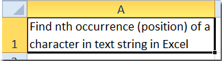
ตัวอย่างเช่นมีประโยคยาวในเซลล์ A1 โปรดดูภาพหน้าจอต่อไปนี้ ตอนนี้คุณต้องหาตำแหน่งที่ 3 หรือตำแหน่งของอักขระ "c" จากสตริงข้อความในเซลล์ A1 แน่นอนคุณสามารถนับอักขระทีละตัวและได้ผลลัพธ์ตำแหน่งที่แน่นอน อย่างไรก็ตามในที่นี้เราจะแนะนำเคล็ดลับง่ายๆในการค้นหาเหตุการณ์ที่ n หรือตำแหน่งของอักขระเฉพาะจากสตริงข้อความในเซลล์


ค้นหาลำดับที่ n (ตำแหน่ง) ของอักขระในเซลล์ด้วยสูตร Find

มีสูตรค้นหาสองสูตรที่ช่วยให้คุณค้นหาการเกิดครั้งที่ n หรือตำแหน่งของอักขระเฉพาะจากสตริงข้อความในเซลล์ได้อย่างรวดเร็ว

สูตรต่อไปนี้จะแสดงวิธีค้นหา "c" ครั้งที่ 3 ในเซลล์ A1

ค้นหาสูตร 1

ป้อนสูตรในเซลล์ว่าง = FIND ("c", A1, FIND ("c", A1) +2).

doc-find-nth-ตำแหน่งของข้อความ-string2

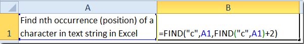
จากนั้นกดปุ่ม เข้าสู่ สำคัญ. ตำแหน่งของตัวอักษรตัวที่สาม“ c” ปรากฏขึ้น

หมายเหตุ: คุณสามารถเปลี่ยน 2 ในสูตรตามความต้องการของคุณ ตัวอย่างเช่นหากคุณต้องการหาตำแหน่งที่สี่ของ "c" คุณสามารถเปลี่ยน 2 เป็น 3 ได้และถ้าคุณต้องการหาตำแหน่งแรกของ "c" คุณจะเปลี่ยน 2 เป็น 0

ค้นหาสูตร 2

ป้อนสูตรในเซลล์ว่าง = ค้นหา (CHAR (1), แทนที่ (A1, "c", CHAR (1), 3))และกด เข้าสู่ กุญแจ

หมายเหตุ: "3" ในสูตรหมายถึง "c" ตัวที่สามคุณสามารถเปลี่ยนได้ตามความต้องการของคุณ


นับครั้งที่คำปรากฏในเซลล์ excel

หากมีคำปรากฏขึ้นหลายครั้งในเซลล์ซึ่งจำเป็นต้องนับโดยปกติคุณอาจนับทีละคำ แต่ถ้าคำนั้นปรากฏขึ้นหลายร้อยครั้งแสดงว่าการนับด้วยตนเองนั้นยุ่งยาก นับครั้งที่คำปรากฏ ฟังก์ชันมา Kutools สำหรับ Excel's ตัวช่วยสูตร กลุ่มสามารถคำนวณจำนวนครั้งที่คำปรากฏในเซลล์ได้อย่างรวดเร็ว ทดลองใช้ฟรีพร้อมคุณสมบัติครบถ้วนใน 30 วัน!
 
Kutools for Excel: มีโปรแกรมเสริม Excel ที่มีประโยชน์มากกว่า 300 รายการให้ทดลองใช้ฟรีโดยไม่มีข้อ จำกัด ใน 30 วัน

> ค้นหาเหตุการณ์ที่ n (ตำแหน่ง) ของอักขระในเซลล์ด้วย VBA

จริงๆแล้วคุณสามารถใช้มาโคร VB เพื่อค้นหาเหตุการณ์ที่ n หรือตำแหน่งของอักขระเฉพาะในเซลล์เดียวได้อย่างง่ายดาย

ขั้นตอนที่ 1: กดปุ่มค้างไว้ ALT + F11 และจะเปิดไฟล์ Microsoft Visual Basic สำหรับแอปพลิเคชัน หน้าต่าง

ขั้นตอนที่ 2: คลิก สิ่งที่ใส่เข้าไป > โมดูลและวางมาโครต่อไปนี้ในหน้าต่างโมดูล

VBA: ค้นหาตำแหน่งที่ n ของอักขระ

Function FindN(sFindWhat As String, _
sInputString As String, N As Integer) As Integer
Dim J As Integer
Application.Volatile
FindN = 0
For J = 1 To N
FindN = InStr(FindN + 1, sInputString, sFindWhat)
If FindN = 0 Then Exit For
Next
End Function

ขั้นตอนที่ 3: ตอนนี้หากคุณต้องการค้นหาตำแหน่งที่แน่นอนของ "c" ที่สามในเซลล์ A1 โปรดป้อนสูตรของ = FindN ("c", A1,3)และกดปุ. ม เข้าสู่ สำคัญ. จากนั้นจะส่งคืนตำแหน่งที่แน่นอนในเซลล์เฉพาะพร้อมกัน


ค้นหาลำดับที่ n (ตำแหน่ง) ของอักขระในเซลล์ด้วย Kutools for Excel

หากคุณไม่ชอบทั้งสูตรและ VBA คุณสามารถลองใช้เครื่องมือที่มีประโยชน์ - Kutools สำหรับ Excelเดียวกันกับที่ สูตร กลุ่มคุณสามารถค้นหายูทิลิตี้ - ค้นหาที่ n ที่เกิดขึ้นของอักขระ เพื่อคืนตำแหน่งที่ n ของอักขระในเซลล์อย่างรวดเร็ว

Kutools สำหรับ Excel, ที่มีมากกว่า 300 ฟังก์ชั่นที่มีประโยชน์ทำให้งานของคุณง่ายขึ้น 

หลังจาก ติดตั้งฟรี Kutools สำหรับ Excel โปรดทำดังนี้:

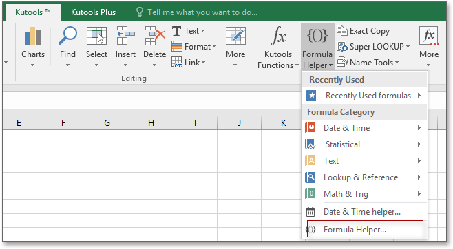
1. เลือกเซลล์ที่คุณต้องการส่งคืนผลลัพธ์แล้วคลิก Kutools > ตัวช่วยสูตร > ตัวช่วยสูตร . ดูภาพหน้าจอ:

2. จากนั้นในการป๊อกกี้ ตัวช่วยสูตร โต้ตอบทำตามด้านล่าง:

1) เลือก ค้นหา จากรายการแบบหล่นลงของ ประเภทสูตร มาตรา;

2) เลือก ค้นหาตำแหน่งที่อักขระปรากฏ Nth ในสตริง in เลือกสูตร มาตรา;

3) เลือกเซลล์ที่มีสตริงที่คุณใช้จากนั้นพิมพ์อักขระที่ระบุและเหตุการณ์ที่ n ในกล่องข้อความใน การป้อนอาร์กิวเมนต์ มาตรา.

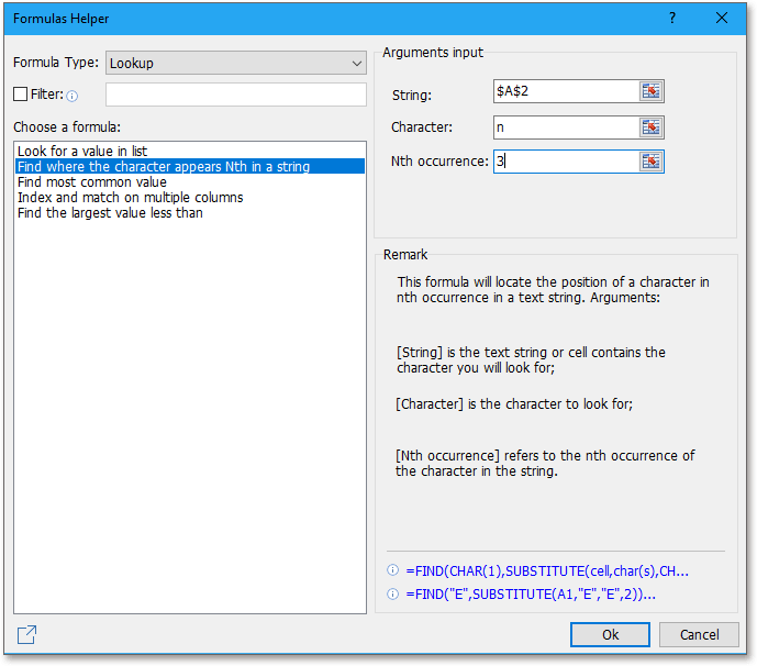
3 คลิก Ok. และคุณจะได้ตำแหน่งของการเกิดอักขระที่ n ในสตริง


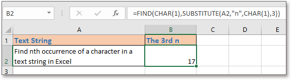
สุดยอดเครื่องมือเพิ่มผลผลิตในสำนักงาน

🤖 Kutools AI ผู้ช่วย: ปฏิวัติการวิเคราะห์ข้อมูลโดยยึดตาม: การดำเนินการที่ชาญฉลาด   |  สร้างรหัส  |  สร้างสูตรที่กำหนดเอง  |  วิเคราะห์ข้อมูลและสร้างแผนภูมิ  |  เรียกใช้ฟังก์ชัน Kutools...
คุณสมบัติยอดนิยม: ค้นหา เน้น หรือระบุรายการที่ซ้ำกัน   |  ลบแถวว่าง   |  รวมคอลัมน์หรือเซลล์โดยไม่สูญเสียข้อมูล   |   รอบโดยไม่มีสูตร ...
การค้นหาขั้นสูง: VLookup หลายเกณฑ์    VLookup หลายค่า  |   VLookup ข้ามหลายแผ่น   |   การค้นหาที่ไม่ชัดเจน ....
รายการแบบเลื่อนลงขั้นสูง: สร้างรายการแบบหล่นลงอย่างรวดเร็ว   |  รายการแบบหล่นลงขึ้นอยู่กับ   |  เลือกหลายรายการแบบหล่นลง ....
ผู้จัดการคอลัมน์: เพิ่มจำนวนคอลัมน์เฉพาะ  |  ย้ายคอลัมน์  |  สลับสถานะการมองเห็นของคอลัมน์ที่ซ่อนอยู่  |  เปรียบเทียบช่วงและคอลัมน์ ...
คุณสมบัติเด่น: กริดโฟกัส   |  มุมมองการออกแบบ   |   บาร์สูตรใหญ่    สมุดงานและตัวจัดการชีต   |  ห้องสมุดทรัพยากร (ข้อความอัตโนมัติ)   |  เลือกวันที่   |  รวมแผ่นงาน   |  เข้ารหัส/ถอดรหัสเซลล์    ส่งอีเมลตามรายการ   |  ซุปเปอร์ฟิลเตอร์   |   ตัวกรองพิเศษ (กรองตัวหนา/ตัวเอียง/ขีดทับ...) ...
ชุดเครื่องมือ 15 อันดับแรก12 ข้อความ เครื่องมือ (เพิ่มข้อความ, ลบอักขระ, ... )   |   50 + แผนภูมิ ประเภท (แผนภูมิ Gantt, ... )   |   40+ ใช้งานได้จริง สูตร (คำนวณอายุตามวันเกิด, ... )   |   19 การแทรก เครื่องมือ (ใส่ QR Code, แทรกรูปภาพจากเส้นทาง, ... )   |   12 การแปลง เครื่องมือ (ตัวเลขเป็นคำ, การแปลงสกุลเงิน, ... )   |   7 ผสานและแยก เครื่องมือ (แถวรวมขั้นสูง, แยกเซลล์, ... )   |   ... และอื่น ๆ

เพิ่มพูนทักษะ Excel ของคุณด้วย Kutools สำหรับ Excel และสัมผัสประสิทธิภาพอย่างที่ไม่เคยมีมาก่อน Kutools สำหรับ Excel เสนอคุณสมบัติขั้นสูงมากกว่า 300 รายการเพื่อเพิ่มประสิทธิภาพและประหยัดเวลา  คลิกที่นี่เพื่อรับคุณสมบัติที่คุณต้องการมากที่สุด...

รายละเอียด


แท็บ Office นำอินเทอร์เฟซแบบแท็บมาที่ Office และทำให้งานของคุณง่ายขึ้นมาก

  • เปิดใช้งานการแก้ไขและอ่านแบบแท็บใน Word, Excel, PowerPoint, ผู้จัดพิมพ์, Access, Visio และโครงการ
  • เปิดและสร้างเอกสารหลายรายการในแท็บใหม่ของหน้าต่างเดียวกันแทนที่จะเป็นในหน้าต่างใหม่
  • เพิ่มประสิทธิภาพการทำงานของคุณ 50% และลดการคลิกเมาส์หลายร้อยครั้งให้คุณทุกวัน!


Comments (28)
No ratings yet. Be the first to rate!
This comment was minimized by the moderator on the site
Your formula to find the Nth occurrence of a character in a string does not work. Using your example, adding 2 to the results of the imbedded find ensures a starting position for the initial find of a position beyond the 1st two c's but changing the +2 to +3 does not yield the position of the 4th "c", it simply starts the search one character deeper into the string and the result is still the 3rd "c". To find the 4th "c" the search must begin beyond the position of the 3rd "c". I look forward to your new solution.
This comment was minimized by the moderator on the site
Hello, David

Yes, as you said, the first formula does not work correctly, you can apply the second formula:
=FIND(CHAR(1),SUBSTITUTE(A2,"c",CHAR(1),2))

Note: The number "2" in the formula means the second "c", if you want to get the third, fourth "c", just change the number 2 to 3,4 as you need.
Please try, hope it can help you!
This comment was minimized by the moderator on the site
Find formula1 is imperfect. It will be a great help if it is removed. I have lost lot of time trying for 4th occurance of "a" in "vedanarayanan" Thanks.
This comment was minimized by the moderator on the site
To handle the exception of the formula, you can use same with if and iserro
=IF(ISERR(FIND("c",A1,FIND("c",A1)+2)),FIND("c",A1,FIND("c",A1)+0),FIND("c",A1,FIND("c",A1)+2))
This comment was minimized by the moderator on the site
"Substitute" lets you find the Nth occurrence of a term, so combine it with "find" as follows (where 5=5th occurrence):

=FIND(CHAR(1),SUBSTITUTE(A1,"c",CHAR(1),5))
This comment was minimized by the moderator on the site
Excellent! I am glad I scrolled up to review other comments after posting my own.
This comment was minimized by the moderator on the site
This is the correct answer! please replace this whole article with this one line of code.....
This comment was minimized by the moderator on the site
The first formula is completely useless and wrong but it works just correct for this example as the first and second "c"s are adjacent. The correct formula is:


For 2nd occurence -
=FIND("c",A1,FIND("c",A1)+1)

For 3rd occurence -
=FIND("c",A1,FIND("c",A1,FIND("c",A1)+1)+1) and so on...
This comment was minimized by the moderator on the site
Absolutely agree. The +2, or +3 etc.....entirely depends on the spacing between the n and (n+1) occurences of "c". Thus you would have to manually adjust for every cell if you were trying to copy this formula down a column for instance. Essentially the same as manually counting.


Ex. Let's try to find the 4th occurrence of "c" in cell A1 using the provided formula. Per the article we should use +3 in our nested FIND function to find the 4th occurrence.


Text in Cell A1:

"cab car abc cole cube"

Manually counting, the 4th occurrence is the "c" in cole in the character position of 13.


=FIND("c",A1,FIND("c",A1)+3)

The nested function, FIND("c",A1) will find the first occurrence of "c" in position 1.

Therefore,

FIND("c",A1)+3 = 1+3 = 4

Plugging that back into our formula,

=FIND("c",A1,FIND("c",A1)+3) = FIND("c",A1,1+3) = FIND("c",A1,4)

This new formula will look for the first occurrence of "c" beginning from character position 4. The 4th character in the string is the space just after cab.

Therefore, the formula will find the "c" in car and return the value of 5 for our formula. As we know from manually counting we are looking for 13 as the output.
This comment was minimized by the moderator on the site
The firs formula works correct in my version, in the note, it has explained how to find the third or forth or nth "c".

Note: You can change the 2 in the formula based on your needs. For example, if you want to find the fourth position of "c", you can change the 2 to 3. And if you want to find the first position of "c", you shuold change 2 to 0.
This comment was minimized by the moderator on the site
Try to find out the position of the second c with the first sentence of my above comment as the string using the first formula. You'll get to know how correct it is!
This comment was minimized by the moderator on the site
Hello all,

I have a text in an Excel cell " BY TRANSFER-NEFT*HDFC0000001*N08745987123546*J0032331*KUMAR--"

I need a function to extract just "N08745987123546"

Thanks
This comment was minimized by the moderator on the site
Hello, do you want to extract the numbers after No and the number of numbers are fixed? If so, you can use Kutools for Exccel's Extract text function, type No????to extract.
This comment was minimized by the moderator on the site
HI ALL,
I have a text in an Excel cell " BY TRANSFER-NEFT*HDHC0065431*N053112345624801*K0038331*krishna--"
I need a function to extract just "N053112345624801"
This comment was minimized by the moderator on the site
Formula 1 doesn't work on fourth, fifth, sixth etc. so (+3,4,5) will always show third position of letter "c" which is 19 second formula is working though.
This comment was minimized by the moderator on the site
Hello all, I have a text in an Excel cell "23 floyd lane, longville,KN 14564" I need a function to extract just "longville" Thanks
This comment was minimized by the moderator on the site
If you must use a function, try: =TRIM(MID(A1,SEARCH(",",A1)+1,SEARCH("!@#",SUBSTITUTE(A1,",","!@#",2))-SEARCH(",",A1)-1)) Otherwise, you might consider Data > Text to Columns > Delimited (using a comma as the separator).
This comment was minimized by the moderator on the site
Try this: =INDEX(SMALL(IF(MID(A1,MATCH(ROW(INDIRECT(1&":"&LEN(A1))),ROW(INDIRECT(1&":"&LEN(A1))),0),1)="c",MATCH(ROW(INDIRECT(1&":"&LEN(A1))),ROW(INDIRECT(1&":"&LEN(A1))),0),""),MATCH(ROW(INDIRECT(1&":"&LEN(A1)-LEN(SUBSTITUTE(A1,"c","")))),ROW(INDIRECT(1&":"&LEN(A1)-LEN(SUBSTITUTE(A1,"c","")))),0)),2) where "c" is the character required and 2 is the position. Note this is an array formula.
This comment was minimized by the moderator on the site
this is simpler: =INDEX(SMALL(IF(MID(A1,ROW(INDIRECT(1&":"&LEN(A1))),1)="c",ROW(INDIRECT(1&":"&LEN(A1))),""),ROW(INDIRECT(1&":"&LEN(A1)-LEN(SUBSTITUTE(A1,"c",""))))),2)
There are no comments posted here yet
Load More
Please leave your comments in English
Posting as Guest
×
Rate this post:
0   Characters
Suggested Locations