วิธีแปลงสูตรเป็นสตริงข้อความใน Excel
โดยปกติ Microsoft Excel จะแสดงผลลัพธ์จากการคำนวณเมื่อคุณป้อนสูตรในเซลล์ อย่างไรก็ตามบางครั้งคุณอาจต้องแสดงเฉพาะสูตรในเซลล์เช่น = CONCATENATE ("000", "- 2")คุณจะจัดการกับมันอย่างไร? มีหลายวิธีในการแก้ปัญหานี้:
แปลงสูตรเป็นสตริงข้อความด้วยคุณสมบัติค้นหาและแทนที่
แปลงสูตรเป็นสตริงข้อความด้วย User Defined Function
แปลงสูตรเป็นสตริงข้อความหรือในทางกลับกันด้วยการคลิกเพียงครั้งเดียว
แปลงสูตรเป็นสตริงข้อความด้วยคุณสมบัติค้นหาและแทนที่
สมมติว่าคุณมีช่วงของสูตรในคอลัมน์ C และคุณต้องแสดงคอลัมน์ที่มีสูตรดั้งเดิม แต่ไม่ใช่ผลลัพธ์จากการคำนวณดังภาพหน้าจอต่อไปนี้:
 |
 |
 |
ในการแก้ปัญหานี้ไฟล์ ค้นหาและแทนที่ คุณสมบัติอาจช่วยคุณได้โปรดทำดังนี้:
1. เลือกเซลล์ผลลัพธ์จากการคำนวณที่คุณต้องการแปลงเป็นสตริงข้อความ
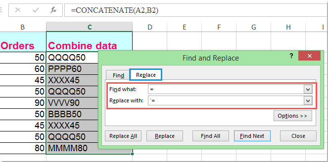
2. จากนั้นกด Ctrl + H คีย์ร่วมกันเพื่อเปิดไฟล์ ค้นหาและแทนที่ กล่องโต้ตอบในกล่องโต้ตอบภายใต้ แทนที่ แท็บป้อนเท่ากับ = ลงชื่อเข้าใช้ สิ่งที่ค้นหา กล่องข้อความและป้อน '= เข้าไปใน แทนที่ด้วย กล่องข้อความดูภาพหน้าจอ:
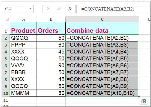
3. จากนั้นคลิก แทนที่ทั้งหมด คุณสามารถดูผลลัพธ์ที่คำนวณทั้งหมดจะถูกแทนที่ด้วยสตริงข้อความสูตรดั้งเดิมดูภาพหน้าจอ:
แปลงสูตรเป็นสตริงข้อความด้วย User Defined Function
รหัส VBA ต่อไปนี้ยังช่วยให้คุณจัดการกับมันได้อย่างง่ายดาย
1. กด อื่น ๆ + F11 ใน Excel และจะเปิดไฟล์ หน้าต่าง Microsoft Visual Basic for Applications.
2. คลิก สิ่งที่ใส่เข้าไป > โมดูลและวางมาโครต่อไปนี้ในไฟล์ หน้าต่างโมดูล.
Function ShowF(Rng As Range)
ShowF = Rng.Formula
End Function
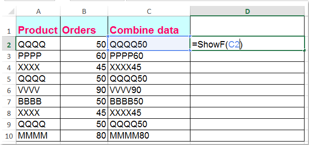
3. ในเซลล์ว่างเช่นเซลล์ D2 ให้ป้อนสูตร = ShowF (C2).
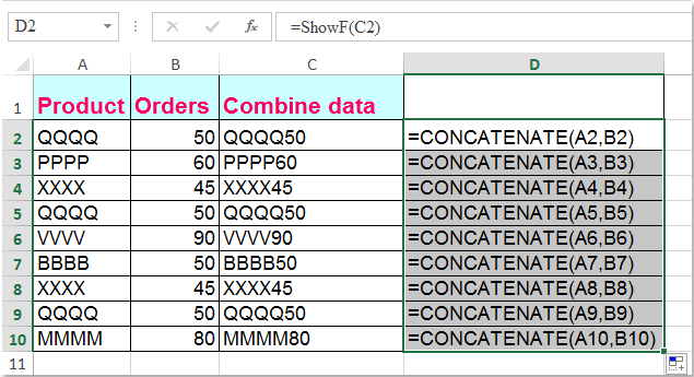
4. จากนั้นคลิกเซลล์ D2 แล้วลาก Fill Handle ![]() ในช่วงที่คุณต้องการ
ในช่วงที่คุณต้องการ
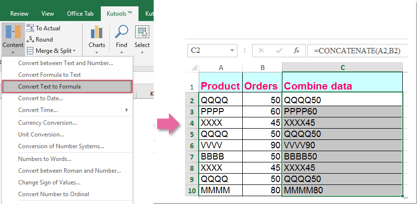
แปลงสูตรเป็นสตริงข้อความหรือในทางกลับกันด้วยการคลิกเพียงครั้งเดียว
ถ้าคุณมี Kutools สำหรับ Excelเดียวกันกับที่ แปลงสูตรเป็นข้อความ คุณสามารถเปลี่ยนหลายสูตรเป็นสตริงข้อความได้ด้วยคลิกเดียว
| Kutools สำหรับ Excel : ด้วย Add-in ของ Excel ที่มีประโยชน์มากกว่า 300 รายการทดลองใช้ฟรีโดยไม่มีข้อ จำกัด ใน 30 วัน. |
หลังจากการติดตั้ง Kutools สำหรับ Excelโปรดทำตามนี้:
1. เลือกสูตรที่คุณต้องการแปลง
2. คลิก Kutools > คอนเทนต์ > แปลงสูตรเป็นข้อความและสูตรที่คุณเลือกได้ถูกแปลงเป็นสตริงข้อความพร้อมกันดูภาพหน้าจอ:

เคล็ดลับ: หากคุณต้องการแปลงสตริงข้อความสูตรกลับไปเป็นผลลัพธ์จากการคำนวณโปรดใช้ยูทิลิตี้แปลงข้อความเป็นสูตรตามภาพหน้าจอต่อไปนี้:
หากคุณต้องการทราบข้อมูลเพิ่มเติมเกี่ยวกับคุณลักษณะนี้โปรดไปที่ แปลงสูตรเป็นข้อความ.
ดาวน์โหลดและทดลองใช้ Kutools for Excel ฟรีทันที!
Demo: แปลงสูตรเป็นสตริงข้อความหรือในทางกลับกันด้วย Kutools for Excel
สุดยอดเครื่องมือเพิ่มผลผลิตในสำนักงาน
เพิ่มพูนทักษะ Excel ของคุณด้วย Kutools สำหรับ Excel และสัมผัสประสิทธิภาพอย่างที่ไม่เคยมีมาก่อน Kutools สำหรับ Excel เสนอคุณสมบัติขั้นสูงมากกว่า 300 รายการเพื่อเพิ่มประสิทธิภาพและประหยัดเวลา คลิกที่นี่เพื่อรับคุณสมบัติที่คุณต้องการมากที่สุด...
")
แท็บ Office นำอินเทอร์เฟซแบบแท็บมาที่ Office และทำให้งานของคุณง่ายขึ้นมาก
- เปิดใช้งานการแก้ไขและอ่านแบบแท็บใน Word, Excel, PowerPoint, ผู้จัดพิมพ์, Access, Visio และโครงการ
- เปิดและสร้างเอกสารหลายรายการในแท็บใหม่ของหน้าต่างเดียวกันแทนที่จะเป็นในหน้าต่างใหม่
- เพิ่มประสิทธิภาพการทำงานของคุณ 50% และลดการคลิกเมาส์หลายร้อยครั้งให้คุณทุกวัน!
")