ไปยังเนื้อหาหลัก

วิธีการแยกสตริงระหว่างสองอักขระที่แตกต่างกันใน Excel

หากคุณมีรายการสตริงใน Excel ซึ่งคุณต้องแยกส่วนของสตริงระหว่างอักขระสองตัวจากภาพด้านล่างที่แสดงวิธีจัดการโดยเร็วที่สุด ที่นี่ฉันจะแนะนำวิธีการบางอย่างเกี่ยวกับการแก้งานนี้

แยกสตริงส่วนระหว่างอักขระสองตัวที่แตกต่างกันด้วยสูตร

แยกสตริงส่วนระหว่างอักขระเดียวกันสองตัวด้วยสูตร

แยกสตริงส่วนระหว่างสองอักขระด้วย Kutools for Excelความคิดที่ดี 3


แยกสตริงส่วนระหว่างอักขระสองตัวที่แตกต่างกันด้วยสูตร

ในการแยกสตริงส่วนระหว่างอักขระสองตัวที่แตกต่างกันคุณสามารถทำได้ดังนี้:

เลือกเซลล์ที่คุณจะวางผลลัพธ์พิมพ์สูตรนี้ =MID(LEFT(A1,FIND(">",A1)-1),FIND("<",A1)+1,LEN(A1))และกด Enter กุญแจ
doc แยกสตริงระหว่างสองอักขระ 1

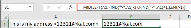
หมายเหตุ: A1 คือเซลล์ข้อความ > และ < เป็นอักขระสองตัวที่คุณต้องการแยกสตริงระหว่าง


แยกสตริงส่วนระหว่างอักขระเดียวกันสองตัวด้วยสูตร

หากคุณต้องการแยกสตริงส่วนระหว่างอักขระเดียวกันสองตัวคุณสามารถทำได้ดังนี้:

เลือกเซลล์ที่คุณจะวางผลลัพธ์พิมพ์สูตรนี้ =SUBSTITUTE(MID(SUBSTITUTE("/" & A3&REPT(" ",6),"/",REPT(",",255)),2*255,255),",","")และกด Enter กุญแจ
doc แยกสตริงระหว่างสองอักขระ 2

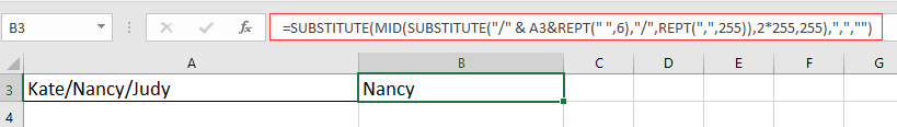
หมายเหตุ A3 คือเซลล์ข้อความ / คืออักขระที่คุณต้องการแยกระหว่าง

แยกสตริงส่วนระหว่างสองอักขระด้วย Kutools for Excel

ถ้าคุณมี Kutools for Excelคุณยังสามารถแยกสตริงส่วนระหว่างสองข้อความ

Kutools สำหรับ Excel, ที่มีมากกว่า 300 ฟังก์ชั่นที่มีประโยชน์ทำให้งานของคุณง่ายขึ้น 

หลังจากการติดตั้ง Kutools สำหรับ Excel โปรดทำดังนี้:(ดาวน์โหลด Kutools for Excel ฟรีทันที!)

1. เลือกเซลล์ที่จะวางสตริงที่แยกออกมาจากนั้นคลิก Kutools > สูตร > ตัวช่วยสูตร.
doc แยกสตริงระหว่างสองอักขระ 3

2 ใน ตัวช่วยสูตร โต้ตอบ, .check ตัวกรอง ช่องทำเครื่องหมายแล้วพิมพ์ "อดีต" ในกล่องข้อความสูตรทั้งหมดเกี่ยวกับการแยกจะแสดงรายการใน เลือกสูตร ส่วนเลือก แยกสตริงระหว่างข้อความที่ระบุจากนั้นไปทางขวา การป้อนอาร์กิวเมนต์ เลือกเซลล์ที่คุณต้องการแยกสตริงย่อยออกมา เซลล์จากนั้นพิมพ์สองข้อความที่คุณต้องการแยก
doc kutools แยกสตริงระหว่างสองข้อความ 2

3 คลิก Okจากนั้นสตริงย่อยระหว่างสองข้อความที่คุณระบุถูกแยกออกแล้วให้ลากที่จับเติมลงเพื่อแยกสตริงย่อยจากแต่ละเซลล์ด้านล่าง
doc kutools แยกสตริงระหว่างสองข้อความ 3

doc kutools แยกสตริงระหว่างสองข้อความ 4

สุดยอดเครื่องมือเพิ่มผลผลิตในสำนักงาน

🤖 Kutools AI ผู้ช่วย: ปฏิวัติการวิเคราะห์ข้อมูลโดยยึดตาม: การดำเนินการที่ชาญฉลาด   |  สร้างรหัส  |  สร้างสูตรที่กำหนดเอง  |  วิเคราะห์ข้อมูลและสร้างแผนภูมิ  |  เรียกใช้ฟังก์ชัน Kutools...
คุณสมบัติยอดนิยม: ค้นหา เน้น หรือระบุรายการที่ซ้ำกัน   |  ลบแถวว่าง   |  รวมคอลัมน์หรือเซลล์โดยไม่สูญเสียข้อมูล   |   รอบโดยไม่มีสูตร ...
การค้นหาขั้นสูง: VLookup หลายเกณฑ์    VLookup หลายค่า  |   VLookup ข้ามหลายแผ่น   |   การค้นหาที่ไม่ชัดเจน ....
รายการแบบเลื่อนลงขั้นสูง: สร้างรายการแบบหล่นลงอย่างรวดเร็ว   |  รายการแบบหล่นลงขึ้นอยู่กับ   |  เลือกหลายรายการแบบหล่นลง ....
ผู้จัดการคอลัมน์: เพิ่มจำนวนคอลัมน์เฉพาะ  |  ย้ายคอลัมน์  |  สลับสถานะการมองเห็นของคอลัมน์ที่ซ่อนอยู่  |  เปรียบเทียบช่วงและคอลัมน์ ...
คุณสมบัติเด่น: กริดโฟกัส   |  มุมมองการออกแบบ   |   บาร์สูตรใหญ่    สมุดงานและตัวจัดการชีต   |  ห้องสมุดทรัพยากร (ข้อความอัตโนมัติ)   |  เลือกวันที่   |  รวมแผ่นงาน   |  เข้ารหัส/ถอดรหัสเซลล์    ส่งอีเมลตามรายการ   |  ซุปเปอร์ฟิลเตอร์   |   ตัวกรองพิเศษ (กรองตัวหนา/ตัวเอียง/ขีดทับ...) ...
ชุดเครื่องมือ 15 อันดับแรก12 ข้อความ เครื่องมือ (เพิ่มข้อความ, ลบอักขระ, ... )   |   50 + แผนภูมิ ประเภท (แผนภูมิ Gantt, ... )   |   40+ ใช้งานได้จริง สูตร (คำนวณอายุตามวันเกิด, ... )   |   19 การแทรก เครื่องมือ (ใส่ QR Code, แทรกรูปภาพจากเส้นทาง, ... )   |   12 การแปลง เครื่องมือ (ตัวเลขเป็นคำ, การแปลงสกุลเงิน, ... )   |   7 ผสานและแยก เครื่องมือ (แถวรวมขั้นสูง, แยกเซลล์, ... )   |   ... และอื่น ๆ

เพิ่มพูนทักษะ Excel ของคุณด้วย Kutools สำหรับ Excel และสัมผัสประสิทธิภาพอย่างที่ไม่เคยมีมาก่อน Kutools สำหรับ Excel เสนอคุณสมบัติขั้นสูงมากกว่า 300 รายการเพื่อเพิ่มประสิทธิภาพและประหยัดเวลา  คลิกที่นี่เพื่อรับคุณสมบัติที่คุณต้องการมากที่สุด...

รายละเอียด


แท็บ Office นำอินเทอร์เฟซแบบแท็บมาที่ Office และทำให้งานของคุณง่ายขึ้นมาก

  • เปิดใช้งานการแก้ไขและอ่านแบบแท็บใน Word, Excel, PowerPoint, ผู้จัดพิมพ์, Access, Visio และโครงการ
  • เปิดและสร้างเอกสารหลายรายการในแท็บใหม่ของหน้าต่างเดียวกันแทนที่จะเป็นในหน้าต่างใหม่
  • เพิ่มประสิทธิภาพการทำงานของคุณ 50% และลดการคลิกเมาส์หลายร้อยครั้งให้คุณทุกวัน!
Comments (35)
No ratings yet. Be the first to rate!
This comment was minimized by the moderator on the site
Bonjour,

je souhaite extraire de ce texte (USD) 934.915765 (30-11-2022) le numero 934.915765, ce que je souhaite c'est faire un extrait de tout ce qui est entre (USD) et (30-11-2022)
This comment was minimized by the moderator on the site
Hi, please try this formula:
=LEFT((MID(I1,FIND(" ",I1)+1,256)),FIND(" ",(MID(I1,FIND(" ",I1)+1,256)),1)-1)
I1 is the cell that you want to extract number.
This comment was minimized by the moderator on the site
Hi, try this formula please:
=IFERROR(MID(A1,FIND("CG",A1),11),IFERROR(MID(A1,FIND("CP",A1),11),IFERROR(MID(A1,FIND("CV",A1),11),IFERROR(MID(A1,FIND("CD",A1),11),IFERROR(MID(A1,FIND("CC",A1),11),MID(A1,FIND("CO",A1),11))))))

If there is no match string, it returns #VALUE! error.
This comment was minimized by the moderator on the site
Hello, can you please help me with extracting a code from a cell? The code is always 11 characters long and it can start with either CC, CP, CV, CO, CG or CD. If it helps, it also ends with a number always. The code does not have a fixed position, it can be in the beginning, middle or end.
I tried this formula =MID(A2,FIND("CP",A2),11) but, as you see, it only finds the ones starting with CP.

An example of what the cell might contain is:
Text text CG1234dh201 text 123 text

Thank you!
This comment was minimized by the moderator on the site
Hi, I have an issue which i am struggling to solve. So I have a number of answers and i want to separate into separate cells.

i.e. A: XYZ|B*: SDR|C: AQS|

I can separate but my issue is there loads of line with the asterisk moving to the correct answer for each question. How do i get my head around this?

I am currently using the below formula

=MID(A5,SEARCH("A:",cell ref)+2,SEARCH("|",A5)-SEARCH(":",cell ref)-1)
This comment was minimized by the moderator on the site
Hi, Mohannmed Faisal, from my understanding, your question is to extract XYZ, SDR and AQS separately into three cells. If so, please use formulas below separately:
=MID(A7,SEARCH("A:",A7)+3,3)
=MID(A7,SEARCH("B*:",A7)+4,3)
=MID(A7,SEARCH("|C:",A7)+4,3)
A7 is the cell that you use to extract.
Hope it help you.
This comment was minimized by the moderator on the site
Bonjour,

J'ai un texte AAMMJJ que je souhaite transformer en JJMMAAAA
This comment was minimized by the moderator on the site
Hi, GG, try this formula =TEXTE(date; "jj/mm/aaaa")
This comment was minimized by the moderator on the site
Hi How to get specific value from description like
Desc: Date: 2022-07-22 23:59:51 Node: VA10TWPSQL026 Type: TSM SM_SERVER_EVENT 2579 Resource: 1700 Message Key: TSM_VA10TWPSQL026

I want to get node value as VA10TWPSQL026
This comment was minimized by the moderator on the site
Hi, Sandhya, if the node value always has a fixed length (14-chars), you can try this formula: =MID(A1,SEARCH("Node",A1)+5,14) hope it do a favor for you.
This comment was minimized by the moderator on the site
Hola,

Me encantan tus foros.

Me podrias ayudar con esto?

Tengo una serie de columnas asi:

U CALIPER R/H/R 1J0615424H Es
N DOOR WINDOW SWITCH R/H/F 8E0959851D5PR Ebbett Audi
N TAILIGHT L/H - LENS & BODY - ON QTR - W/XENON H/LAMP 63217217311 Coombes Johnson European Ltd
U*GUARD R/H/F - REPLACE RET NUT ALSO 5G0821106A (V) Private Purchase

Lo que necesito extraer es el numero de parte de cada celda pero siempre esta en una posicion diferente, por ejemplo de la primer celda necesito solo 1J0615424H, de la segunda necesito extraer 8E0959851D5PR, de la tercera 63217217311 y de la ultima 5G0821106A

Muchas gracias

Anderson
This comment was minimized by the moderator on the site
Hallo,

Ik moet een stuk tekst extraheren uit een cel, maar kom er niet aan uit.

51420647 Ondersteuner Kringdirectie (Unfilled)
P_00040501 Productmanager Wendbare Pool Bedrijven (Unfilled)

De tekst die ik nodig heb ik is het middelste deel tussen de cijfers en (unfilled).
Welke formuler kan ik hiervoor gebruiken?
This comment was minimized by the moderator on the site
HelloI have an issue where I am trying to extract a number from a set of text and numbers in excel. This is an excerpt from the data I have:AUS23-7W
GER490-8W
MEX114-2M
MEX444-5M
MEX331-3W
US118-15W
ARG572-16W
Japan122-6W
Japan526-13W
ARG585-7W
Japan398-16W
Japan320-15W
ARG141-3Mo
Canada329-5W
US421-17Mo
Canada427-14W
I need to be able to extract just the number to the right of the dash. For example, I need Japan320-15W to return just the 15 in its own column. Is there a formula you could provide me with that can accomplish this? Many thanks!

This comment was minimized by the moderator on the site
Hello, Duggled, to solve your job, just need two steps. Firstly, select the text strings, and apply Text to Columns under Data tab, choose Delimited > Other, and type - into the textbox beside Other option, click Finish. In this step, your data has been split into two columns by deliliter -. Secondly, use the formula  =SUMPRODUCT(MID(0&B1, LARGE(INDEX(ISNUMBER(--MID(B1, ROW(INDIRECT("1:"&LEN(B1))), 1)) * ROW(INDIRECT("1:"&LEN(B1))), 0), ROW(INDIRECT("1:"&LEN(B1))))+1, 1) * 10^ROW(INDIRECT("1:"&LEN(B1)))/10)(A1 is the cell that you want to extract the number from, here you change it to your second column cell)then the numbers after - have been extracted. Or in the second step, you can apply VBA, or our handy tool, for more details, please visit:https://www.extendoffice.com/documents/excel/1622-excel-extract-number-from-string.html
This comment was minimized by the moderator on the site
This formula works well for pretty much everything except these data :MEX114-2M
MEX444-5M
MEX373-15M
MEX540-8M
MEX396-11M
MEX386-10M
MEX369-14M
MEX446-3M
MEX75-12M
MEX372-3M
MEX178-6M
MEX510-7M
MEX361-17M
MEX501-13M
MEX221-17M
Is there any way you could revise that formula to include these? Thank you so much!
This comment was minimized by the moderator on the site
Hi! Sorry if I reposted this and thank you so much for the formula.
But I'm not sure how to do this, I have this in a cell:

random comment;24/nov/21 2:34 PM;random ID;3240

and I need to get in separate cells the date without the hour, like 24/nov/21 . And, in another cell, the last numer; in this case 3240 (The format is alway the same, and the date is always 9 characters long, the only thing that might change is the last number, as is the number of seconds it took to do something)

How should I do it?
Thank you!! 
This comment was minimized by the moderator on the site
Hi, to extract date, please use formula =MID(A1,16,9), A1 is the cell that the original data places, to extract ID number, please use formula =MID(A1,44,10),, for more details, you can refer to this articel https://www.extendoffice.com/documents/excel/3639-excel-extract-part-of-string.html
There are no comments posted here yet
Load More
Please leave your comments in English
Posting as Guest
×
Rate this post:
0   Characters
Suggested Locations