ไปยังเนื้อหาหลัก

วิธีการแยกค่าในรายการหนึ่งจากรายการอื่นใน Excel

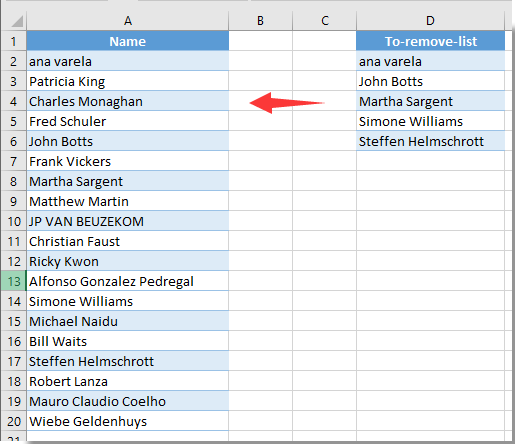
สมมติว่าคุณมีรายการข้อมูลสองรายการตามภาพหน้าจอด้านซ้ายที่แสดง ตอนนี้คุณต้องลบหรือยกเว้นชื่อในคอลัมน์ A ถ้าชื่อที่มีอยู่ในคอลัมน์ D จะบรรลุได้อย่างไร? และจะเกิดอะไรขึ้นถ้าทั้งสองรายการพบในแผ่นงานสองแผ่น? บทความนี้มีสองวิธีสำหรับคุณ

ไม่รวมค่าในรายการหนึ่งจากอีกรายการด้วยสูตร

แยกค่าในรายการหนึ่งออกจากรายการอื่นอย่างรวดเร็วด้วย Kutools for Excel


ไม่รวมค่าในรายการหนึ่งจากอีกรายการด้วยสูตร

คุณสามารถใช้สูตรต่อไปนี้เพื่อให้บรรลุ กรุณาดำเนินการดังนี้

1. เลือกเซลล์ว่างที่อยู่ติดกับเซลล์แรกของรายการที่คุณต้องการลบจากนั้นป้อนสูตร = COUNTIF ($ D $ 2: $ D $ 6, A2) ลงในแถบสูตรแล้วกดปุ่ม เข้าสู่ สำคัญ. ดูภาพหน้าจอ:

หมายเหตุ: ในสูตร $ D $ 2: $ D $ 6 คือรายการที่คุณจะลบค่าตาม A2 คือเซลล์แรกของรายการที่คุณจะลบ โปรดเปลี่ยนตามที่คุณต้องการ

2. เลือกเซลล์ผลลัพธ์ต่อไปลาก Fill Handle ลงไปจนกระทั่งถึงเซลล์สุดท้ายของรายการ ดูภาพหน้าจอ:

3. เลือกรายการผลลัพธ์จากนั้นคลิก ข้อมูล > เรียงลำดับ A ถึง Z.

จากนั้นคุณจะเห็นรายการถูกจัดเรียงตามภาพด้านล่างที่แสดง

4. ตอนนี้เลือกแถวทั้งหมดของชื่อที่มีผลลัพธ์ 1 คลิกขวาช่วงที่เลือกแล้วคลิก ลบ เพื่อลบออก

ตอนนี้คุณได้ยกเว้นค่าในรายการหนึ่งตามอีกรายการหนึ่งแล้ว

หมายเหตุ: หากตำแหน่ง "to-remove-list" อยู่ในช่วง A2: A6 ของแผ่นงานอื่นเช่น Sheet2 โปรดใช้สูตรนี้ = IF (ISERROR (VLOOKUP (A2, Sheet2! $ A $ 2: $ A $ 6,1, FALSE)), "Keep", "Delete") เพื่อรับทั้งหมด เก็บ และ ลบ ไปข้างหน้าเพื่อเรียงลำดับรายการผลลัพธ์จาก Ato Z จากนั้นลบแถวชื่อทั้งหมดด้วยตนเองที่มีผลลัพธ์ Delete ในแผ่นงานปัจจุบัน


แยกค่าในรายการหนึ่งออกจากรายการอื่นอย่างรวดเร็วด้วย Kutools for Excel

ส่วนนี้จะแนะนำไฟล์ เลือกเซลล์เดียวกันและต่างกัน ประโยชน์ของ Kutools สำหรับ Excel เพื่อแก้ปัญหานี้ กรุณาดำเนินการดังนี้

ก่อนที่จะใช้ Kutools สำหรับ Excelโปรด ดาวน์โหลดและติดตั้งในตอนแรก.

1 คลิก Kutools > เลือก > เลือกเซลล์เดียวกันและต่างกัน. ดูภาพหน้าจอ:

2 ใน เลือกเซลล์เดียวกันและต่างกัน คุณต้อง:

  • 2.1 เลือกรายการที่คุณจะลบค่าออกจากไฟล์ ค้นหาค่าใน กล่อง;
  • 2.2 เลือกรายการที่คุณจะลบค่าตามใน ตามที่ กล่อง;
  • 2.3 เลือก เซลล์เดี่ยว ตัวเลือกใน อยู่บนพื้นฐานของ มาตรา;
  • 2.4 คลิกปุ่ม OK ปุ่ม. ดูภาพหน้าจอ:

3. จากนั้นกล่องโต้ตอบจะปรากฏขึ้นเพื่อบอกจำนวนเซลล์ที่ถูกเลือกโปรดคลิกที่ OK ปุ่ม

4. ตอนนี้ค่าในคอลัมน์ A ถูกเลือกหากมีอยู่ในคอลัมน์ D คุณสามารถกดปุ่ม ลบ คีย์เพื่อลบด้วยตนเอง

  หากคุณต้องการทดลองใช้ยูทิลิตีนี้ฟรี (30 วัน) กรุณาคลิกเพื่อดาวน์โหลดแล้วไปใช้การดำเนินการตามขั้นตอนข้างต้น


แยกค่าในรายการหนึ่งออกจากรายการอื่นอย่างรวดเร็วด้วย Kutools for Excel


บทความที่เกี่ยวข้อง:

สุดยอดเครื่องมือเพิ่มผลผลิตในสำนักงาน

🤖 Kutools AI ผู้ช่วย: ปฏิวัติการวิเคราะห์ข้อมูลโดยยึดตาม: การดำเนินการที่ชาญฉลาด   |  สร้างรหัส  |  สร้างสูตรที่กำหนดเอง  |  วิเคราะห์ข้อมูลและสร้างแผนภูมิ  |  เรียกใช้ฟังก์ชัน Kutools...
คุณสมบัติยอดนิยม: ค้นหา เน้น หรือระบุรายการที่ซ้ำกัน   |  ลบแถวว่าง   |  รวมคอลัมน์หรือเซลล์โดยไม่สูญเสียข้อมูล   |   รอบโดยไม่มีสูตร ...
การค้นหาขั้นสูง: VLookup หลายเกณฑ์    VLookup หลายค่า  |   VLookup ข้ามหลายแผ่น   |   การค้นหาที่ไม่ชัดเจน ....
รายการแบบเลื่อนลงขั้นสูง: สร้างรายการแบบหล่นลงอย่างรวดเร็ว   |  รายการแบบหล่นลงขึ้นอยู่กับ   |  เลือกหลายรายการแบบหล่นลง ....
ผู้จัดการคอลัมน์: เพิ่มจำนวนคอลัมน์เฉพาะ  |  ย้ายคอลัมน์  |  สลับสถานะการมองเห็นของคอลัมน์ที่ซ่อนอยู่  |  เปรียบเทียบช่วงและคอลัมน์ ...
คุณสมบัติเด่น: กริดโฟกัส   |  มุมมองการออกแบบ   |   บาร์สูตรใหญ่    สมุดงานและตัวจัดการชีต   |  ห้องสมุดทรัพยากร (ข้อความอัตโนมัติ)   |  เลือกวันที่   |  รวมแผ่นงาน   |  เข้ารหัส/ถอดรหัสเซลล์    ส่งอีเมลตามรายการ   |  ซุปเปอร์ฟิลเตอร์   |   ตัวกรองพิเศษ (กรองตัวหนา/ตัวเอียง/ขีดทับ...) ...
ชุดเครื่องมือ 15 อันดับแรก12 ข้อความ เครื่องมือ (เพิ่มข้อความ, ลบอักขระ, ... )   |   50 + แผนภูมิ ประเภท (แผนภูมิ Gantt, ... )   |   40+ ใช้งานได้จริง สูตร (คำนวณอายุตามวันเกิด, ... )   |   19 การแทรก เครื่องมือ (ใส่ QR Code, แทรกรูปภาพจากเส้นทาง, ... )   |   12 การแปลง เครื่องมือ (ตัวเลขเป็นคำ, การแปลงสกุลเงิน, ... )   |   7 ผสานและแยก เครื่องมือ (แถวรวมขั้นสูง, แยกเซลล์, ... )   |   ... และอื่น ๆ

เพิ่มพูนทักษะ Excel ของคุณด้วย Kutools สำหรับ Excel และสัมผัสประสิทธิภาพอย่างที่ไม่เคยมีมาก่อน Kutools สำหรับ Excel เสนอคุณสมบัติขั้นสูงมากกว่า 300 รายการเพื่อเพิ่มประสิทธิภาพและประหยัดเวลา  คลิกที่นี่เพื่อรับคุณสมบัติที่คุณต้องการมากที่สุด...

รายละเอียด


แท็บ Office นำอินเทอร์เฟซแบบแท็บมาที่ Office และทำให้งานของคุณง่ายขึ้นมาก

  • เปิดใช้งานการแก้ไขและอ่านแบบแท็บใน Word, Excel, PowerPoint, ผู้จัดพิมพ์, Access, Visio และโครงการ
  • เปิดและสร้างเอกสารหลายรายการในแท็บใหม่ของหน้าต่างเดียวกันแทนที่จะเป็นในหน้าต่างใหม่
  • เพิ่มประสิทธิภาพการทำงานของคุณ 50% และลดการคลิกเมาส์หลายร้อยครั้งให้คุณทุกวัน!
Comments (16)
No ratings yet. Be the first to rate!
This comment was minimized by the moderator on the site
"foruma contains an error!"
Wondeful help...
This comment was minimized by the moderator on the site
the function is correct: maybe you have Excel in a different language than english. Change the function names in that way. :)
This comment was minimized by the moderator on the site
Thank you for this. It solved my problem of wanting to include only companies from a list
This comment was minimized by the moderator on the site
This formula subtracts list in column B from list in columnA:=FILTER(IFNA(MATCH(A2:A12,B2:B6,0),A2:A12),ISNUMBER(IFNA(MATCH(A2:A12,B2:B6,0),A2:A12))=FALSE)
This comment was minimized by the moderator on the site
But this one's simpler (Subtracts list in A2:A20 from list in D2:D6):=FILTER(A2:A20,ISERROR(MATCH(A2:A20,D2:D6,0))=TRUE)
This comment was minimized by the moderator on the site
Keith,

This formula was incredibly helpful (even more helpful than the actual blog post!) You're a life saver! This formula gets really powerful if you use it in dynamic arrays.
This comment was minimized by the moderator on the site
what if I have multiple columns?
This comment was minimized by the moderator on the site
Depends on the structure of your lists, but if you want to exclude several lists Y and Z from a single big list X, try something like this:
=FILTER(X3:X21,ISERROR(MATCH(X3:X21,Y3:Y6,0))*ISERROR(MATCH(X3:X21,Z3:Z5,0))=1)
this returns listX minus listY and listZ.
The "ISERROR(MATCH(X3:X21,Y3:Y6,0))" returns "TRUE" if an item in listX is missing from listY, likewise ISERROR(MATCH(X3:X21,Z3:Z5,0)) for listX and listZ.
A quirk of Excel is that "=TRUE*TRUE" will return "1". In fact, any number of TRUEs multiplied will return "1", but include a single FALSE and it will return "0".
So the FILTER will return only those items from the list where all the "ISERROR(MATCH....." formulae are TRUE.
For each additional list of items to exclude, add an extra *ISERROR(MATCH(listX,list_exclude,0)) before the "=1)"
This comment was minimized by the moderator on the site
You could try a filter of a filter:=FILTER(A2:A20,ISERROR(MATCH(A2:A20,FILTER(Array2,Include_criteria2)))=TRUE)
This comment was minimized by the moderator on the site
Apologies, that should read "Subtracts list in D2:D6 from list in A2:A20."
This comment was minimized by the moderator on the site
Apologies, that should read "Subtracts list in D2:D6 from list in A2:A20."
This comment was minimized by the moderator on the site
Apologies, that should read "Subtracts list in D2:D6 from list in A2:A20"
This comment was minimized by the moderator on the site
Good find. Thank you for this clever workaround. I thought was only possible via macros.
Possible to do the same using method 1, for a range consisting in two columns. i.e City, State in col D2:E20 while my A2:C1000 (B:C has city,state) has the set I need to get marked?
tried this did not work: =COUNTIF($D$2:$E$20,B2:C2). Unless you have another wonderful guide.
This comment was minimized by the moderator on the site
Как безграмотный человек писал эту статью? Тот, кто русский язык не учил, ни одной книги не прочел и не общался в социуме никогда? Уже с самого начала статьи обороты почти в каждом предложении такие, что на голову не натянешь. Зачем писать, если не умеешь писать?
This comment was minimized by the moderator on the site
I receive other values in the COUNTIF column like 2 but also higher numbers other than 0 and 1. What does that mean?
This comment was minimized by the moderator on the site
The values you get in the COUNTIF column are equal to the number of occurrences of the element in the right column. For example, if you have 5 displayed against a cell in the Name column, it means that this name was found in the To-remove-list not one, but five times.
There are no comments posted here yet
Please leave your comments in English
Posting as Guest
×
Rate this post:
0   Characters
Suggested Locations