ไปยังเนื้อหาหลัก

วิธีค้นหาค่าที่ไม่ใช่ศูนย์แรกและส่งคืนส่วนหัวคอลัมน์ที่เกี่ยวข้องใน Excel

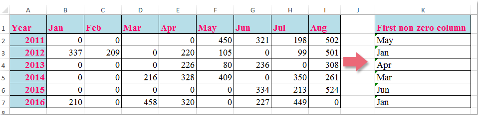
สมมติว่าคุณมีช่วงของข้อมูลตอนนี้คุณต้องการส่งคืนส่วนหัวของคอลัมน์ในแถวนั้นซึ่งค่าที่ไม่ใช่ศูนย์แรกเกิดขึ้นตามภาพหน้าจอต่อไปนี้บทความนี้ฉันจะแนะนำสูตรที่มีประโยชน์สำหรับคุณในการจัดการกับงานนี้ ใน Excel

การค้นหาเอกสารก่อนไม่ใช่ศูนย์ 1

ค้นหาค่าที่ไม่ใช่ศูนย์แรกและส่งคืนส่วนหัวคอลัมน์ที่เกี่ยวข้องด้วยสูตร


ลูกศรสีฟ้าฟองขวา ค้นหาค่าที่ไม่ใช่ศูนย์แรกและส่งคืนส่วนหัวคอลัมน์ที่เกี่ยวข้องด้วยสูตร

หากต้องการส่งคืนส่วนหัวคอลัมน์ของค่าที่ไม่ใช่ศูนย์แรกในแถวสูตรต่อไปนี้อาจช่วยคุณได้โปรดดำเนินการดังนี้:

ใส่สูตรนี้: =INDEX($B$1:$I$1,MATCH(TRUE,INDEX(B2:I2<>0,),0)) ลงในเซลล์ว่างที่คุณต้องการค้นหาผลลัพธ์ K2ตัวอย่างเช่นจากนั้นลากที่จับเติมลงไปที่เซลล์ที่คุณต้องการใช้สูตรนี้และส่วนหัวคอลัมน์ที่เกี่ยวข้องทั้งหมดของค่าที่ไม่ใช่ศูนย์แรกจะถูกส่งกลับตามภาพหน้าจอต่อไปนี้:

การค้นหาเอกสารก่อนไม่ใช่ศูนย์ 2

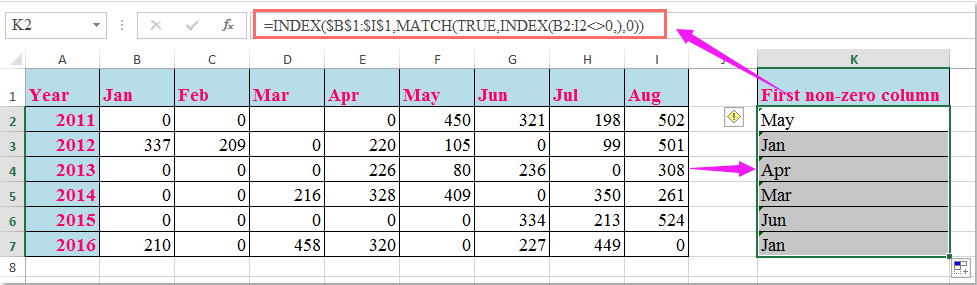
หมายเหตุ: ในสูตรข้างต้น B1: I1 คือส่วนหัวของคอลัมน์ที่คุณต้องการส่งคืน B2: I2 คือข้อมูลแถวที่คุณต้องการค้นหาค่าที่ไม่ใช่ศูนย์แรก

สุดยอดเครื่องมือเพิ่มผลผลิตในสำนักงาน

🤖 Kutools AI ผู้ช่วย: ปฏิวัติการวิเคราะห์ข้อมูลโดยยึดตาม: การดำเนินการที่ชาญฉลาด   |  สร้างรหัส  |  สร้างสูตรที่กำหนดเอง  |  วิเคราะห์ข้อมูลและสร้างแผนภูมิ  |  เรียกใช้ฟังก์ชัน Kutools...
คุณสมบัติยอดนิยม: ค้นหา เน้น หรือระบุรายการที่ซ้ำกัน   |  ลบแถวว่าง   |  รวมคอลัมน์หรือเซลล์โดยไม่สูญเสียข้อมูล   |   รอบโดยไม่มีสูตร ...
การค้นหาขั้นสูง: VLookup หลายเกณฑ์    VLookup หลายค่า  |   VLookup ข้ามหลายแผ่น   |   การค้นหาที่ไม่ชัดเจน ....
รายการแบบเลื่อนลงขั้นสูง: สร้างรายการแบบหล่นลงอย่างรวดเร็ว   |  รายการแบบหล่นลงขึ้นอยู่กับ   |  เลือกหลายรายการแบบหล่นลง ....
ผู้จัดการคอลัมน์: เพิ่มจำนวนคอลัมน์เฉพาะ  |  ย้ายคอลัมน์  |  สลับสถานะการมองเห็นของคอลัมน์ที่ซ่อนอยู่  |  เปรียบเทียบช่วงและคอลัมน์ ...
คุณสมบัติเด่น: กริดโฟกัส   |  มุมมองการออกแบบ   |   บาร์สูตรใหญ่    สมุดงานและตัวจัดการชีต   |  ห้องสมุดทรัพยากร (ข้อความอัตโนมัติ)   |  เลือกวันที่   |  รวมแผ่นงาน   |  เข้ารหัส/ถอดรหัสเซลล์    ส่งอีเมลตามรายการ   |  ซุปเปอร์ฟิลเตอร์   |   ตัวกรองพิเศษ (กรองตัวหนา/ตัวเอียง/ขีดทับ...) ...
ชุดเครื่องมือ 15 อันดับแรก12 ข้อความ เครื่องมือ (เพิ่มข้อความ, ลบอักขระ, ... )   |   50 + แผนภูมิ ประเภท (แผนภูมิ Gantt, ... )   |   40+ ใช้งานได้จริง สูตร (คำนวณอายุตามวันเกิด, ... )   |   19 การแทรก เครื่องมือ (ใส่ QR Code, แทรกรูปภาพจากเส้นทาง, ... )   |   12 การแปลง เครื่องมือ (ตัวเลขเป็นคำ, การแปลงสกุลเงิน, ... )   |   7 ผสานและแยก เครื่องมือ (แถวรวมขั้นสูง, แยกเซลล์, ... )   |   ... และอื่น ๆ

เพิ่มพูนทักษะ Excel ของคุณด้วย Kutools สำหรับ Excel และสัมผัสประสิทธิภาพอย่างที่ไม่เคยมีมาก่อน Kutools สำหรับ Excel เสนอคุณสมบัติขั้นสูงมากกว่า 300 รายการเพื่อเพิ่มประสิทธิภาพและประหยัดเวลา  คลิกที่นี่เพื่อรับคุณสมบัติที่คุณต้องการมากที่สุด...

รายละเอียด


แท็บ Office นำอินเทอร์เฟซแบบแท็บมาที่ Office และทำให้งานของคุณง่ายขึ้นมาก

  • เปิดใช้งานการแก้ไขและอ่านแบบแท็บใน Word, Excel, PowerPoint, ผู้จัดพิมพ์, Access, Visio และโครงการ
  • เปิดและสร้างเอกสารหลายรายการในแท็บใหม่ของหน้าต่างเดียวกันแทนที่จะเป็นในหน้าต่างใหม่
  • เพิ่มประสิทธิภาพการทำงานของคุณ 50% และลดการคลิกเมาส์หลายร้อยครั้งให้คุณทุกวัน!
Comments (15)
No ratings yet. Be the first to rate!
This comment was minimized by the moderator on the site
Hello, my problem is: a have value 1,2,3,4,...50 that are the number of month. How to denormalize month into real datum. Thank you in advance a lot!!!
This comment was minimized by the moderator on the site
Does anyone know what you would do if your cell that contains a zero has a formula in it? When I use this formula, I end up with whatever the first column header is regardless of whether it is zero or not.
This comment was minimized by the moderator on the site
E como faço pra procurar o primeiro valor diferente de zero da esquerda pra direita?
This comment was minimized by the moderator on the site
Hello, Matheus
If you want to return the first non-zero value from a row, please apply the below formula:
=INDEX(B2:F2,MATCH(TRUE,INDEX(B2:F2<>0,),0))
Please have a try, hope it can help you!
This comment was minimized by the moderator on the site
What if you needed the last non-zero value in an array?

P.S. This was really helpful, thank you so much!
This comment was minimized by the moderator on the site
Hello, Ali,
To get the column header based on the last non-zero value, please apply the below formula, see screenshot:
=INDEX($B$1:$H$1,MAX((COLUMN(B2:H2)-MIN(COLUMN(B2:H2))+1)*(B2:H2<>0)))
Please remember to press Ctrl+Shift+Enter key together.
https://www.extendoffice.com/images/stories/comments/comment-skyyang/doc-last-non-zero.png
Please try, hope it can help you!
This comment was minimized by the moderator on the site
The formula is super helpful and helped me sorted out the situation! Thanks!!! Is there any chance you may please help to also explain how it works?
This comment was minimized by the moderator on the site
How do you look up for the second,third and fourth non-zero value?
This comment was minimized by the moderator on the site
Hello, Robert,
To lookup the second, third or fourth non-zero values and return their columns, please apply the below formula: (After pasting the formula, please press Ctr + Shift + Enter keys together.)
=INDEX($B$1:$I$1,SMALL(IF(B2:I2<>0, COLUMN(B2:I2)-COLUMN(A2)),2))


Note: To extract the third or fourth result, you just need to change the number 2 to 3,4 as you need.

Please have a try, hope it can help you!
This comment was minimized by the moderator on the site
CAN U EXPLIAN HOW THIS FORMULA WORKS
This comment was minimized by the moderator on the site
Hello Priya,I am glad to help. I will separate the formula = INDEX($B$1:$I$1,MATCH(TRUE,INDEX(B2:I2<>0,),0)) into 3 parts, and explain the formula to you step by step.
First, let us see the inner-most formula =INDEX(B2:I2<>0,). This formula returns an array of TRUE and FALSE whether the values of range B2:I2 are equal to 0. Please see the screenshot 1, formula =INDEX(B2:I2<>0,) returns {FALSE,FALSE,FALSE,FALSE,TRUE,TRUE,TRUE,TRUE}.
Second, =MATCH(TRUE,INDEX(B2:I2<>0,),0) =MATCH(TRUE, {FALSE,FALSE,FALSE,FALSE,TRUE,TRUE,TRUE,TRUE}, 0). It returns the position of the first value "TRUE", while 0 in the formula means an exact match. We can see that the first value "TRUE" occurs at the 5th position of the array. Then the second formula returns 5. See the screenshot 2.
Finally,  =INDEX(B1:I1,MATCH(TRUE,INDEX(B2:I2<>0,),0))=INDEX(B1:I1,5). It returns the 5th value of the array B1:I1. We can see in the screenshot that the value is "May". So the final formula returns "May". 
PS: To drag the fill handle down the formula to get the rest of the results, we must make the range B1:I1 absolute. So we add $ to range B1:I1 to keep it absolute. 
Hope my explanation can solve your puzzle. Have a nice day.
Sincerely,Mandy
This comment was minimized by the moderator on the site
Thank you Mandy for illustrating it in detail.
Kindly guide how to get the last non zero value from same formula instead of first non zero value.
Will Match work for that or not?
This comment was minimized by the moderator on the site
Hi MandyZhou,

Thank you for the explanation!
I have a follow-up question.
How would the formula change if you had to look up the year too?
So in the above example, let's assume that column J is 'Year' and that in cell J2 is written '2015'.
And in cell K2 I would need the column header for the first non-zero value of the year in L2 (year 2015, so I would need to find 'Jun' in cell K2).

Thanks in advance for your help!
Jason
This comment was minimized by the moderator on the site
How can I return the second and third, etc non zero value? Your formula is amazing but I am trying to search more keywords from a text so sometimes they are 2 or 3 in the same sentence
This comment was minimized by the moderator on the site
se volessi "l'ultimo" Valore Diverso Da Zero E Restituire L'intestazione Della Colonna Corrispondente Con La Formula?
There are no comments posted here yet
Please leave your comments in English
Posting as Guest
×
Rate this post:
0   Characters
Suggested Locations