ไปยังเนื้อหาหลัก

วิธีนับค่าที่ไม่ซ้ำตามคอลัมน์อื่นใน Excel

doc นับไม่ซ้ำตามเกณฑ์ 1

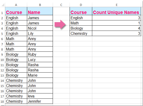
อาจเป็นเรื่องปกติที่เราจะนับค่าที่ไม่ซ้ำกันในคอลัมน์เดียว แต่ในบทความนี้ฉันจะพูดถึงวิธีการนับค่าที่ไม่ซ้ำกันตามคอลัมน์อื่น ตัวอย่างเช่นฉันมีข้อมูลสองคอลัมน์ต่อไปนี้ตอนนี้ฉันต้องการนับชื่อเฉพาะในคอลัมน์ B ตามเนื้อหาของคอลัมน์ A เพื่อให้ได้ผลลัพธ์ต่อไปนี้:

นับค่าที่ไม่ซ้ำกันตามคอลัมน์อื่นด้วยสูตรอาร์เรย์


ลูกศรสีฟ้าฟองขวา นับค่าที่ไม่ซ้ำกันตามคอลัมน์อื่นด้วยสูตรอาร์เรย์

เพื่อแก้ปัญหานี้สูตรต่อไปนี้สามารถช่วยคุณได้โปรดทำดังนี้:

1. ใส่สูตรนี้: =SUMPRODUCT((($A$2:$A$18=D2))/COUNTIFS($A$2:$A$18,$A$2:$A$18&"",$B$2:$B$18,$B$2:$B$18&"")) ลงในเซลล์ว่างที่คุณต้องการใส่ผลลัพธ์ E2ตัวอย่างเช่น จากนั้นกด Ctrl + Shift + Enter คีย์เข้าด้วยกันเพื่อให้ได้ผลลัพธ์ที่ถูกต้องดูภาพหน้าจอ:

doc นับไม่ซ้ำตามเกณฑ์ 2

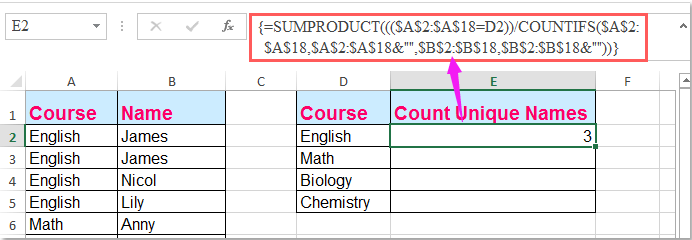
หมายเหตุ: ในสูตรข้างต้น: A2: A18 คือข้อมูลคอลัมน์ที่คุณนับค่าที่ไม่ซ้ำกันตาม B2: B18 คือคอลัมน์ที่คุณต้องการนับค่าเฉพาะ D2 มีเกณฑ์ที่คุณนับไม่ซ้ำกันตาม

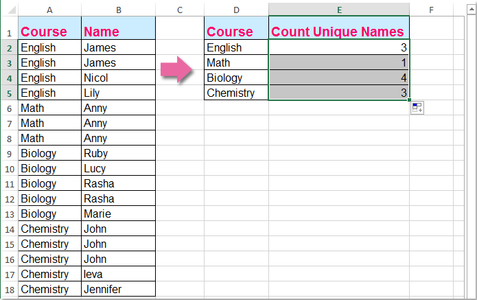
2. จากนั้นลากที่จับเติมลงเพื่อรับค่าเฉพาะของเกณฑ์ที่เกี่ยวข้อง ดูภาพหน้าจอ:

doc นับไม่ซ้ำตามเกณฑ์ 3


บทความที่เกี่ยวข้อง:

วิธีนับจำนวนค่าที่ไม่ซ้ำกันในช่วงใน Excel

วิธีการนับค่าที่ไม่ซ้ำกันในคอลัมน์ที่กรองแล้วใน Excel

จะนับค่าที่เหมือนกันหรือซ้ำกันเพียงครั้งเดียวในคอลัมน์ได้อย่างไร?

สุดยอดเครื่องมือเพิ่มผลผลิตในสำนักงาน

🤖 Kutools AI ผู้ช่วย: ปฏิวัติการวิเคราะห์ข้อมูลโดยยึดตาม: การดำเนินการที่ชาญฉลาด   |  สร้างรหัส  |  สร้างสูตรที่กำหนดเอง  |  วิเคราะห์ข้อมูลและสร้างแผนภูมิ  |  เรียกใช้ฟังก์ชัน Kutools...
คุณสมบัติยอดนิยม: ค้นหา เน้น หรือระบุรายการที่ซ้ำกัน   |  ลบแถวว่าง   |  รวมคอลัมน์หรือเซลล์โดยไม่สูญเสียข้อมูล   |   รอบโดยไม่มีสูตร ...
การค้นหาขั้นสูง: VLookup หลายเกณฑ์    VLookup หลายค่า  |   VLookup ข้ามหลายแผ่น   |   การค้นหาที่ไม่ชัดเจน ....
รายการแบบเลื่อนลงขั้นสูง: สร้างรายการแบบหล่นลงอย่างรวดเร็ว   |  รายการแบบหล่นลงขึ้นอยู่กับ   |  เลือกหลายรายการแบบหล่นลง ....
ผู้จัดการคอลัมน์: เพิ่มจำนวนคอลัมน์เฉพาะ  |  ย้ายคอลัมน์  |  สลับสถานะการมองเห็นของคอลัมน์ที่ซ่อนอยู่  |  เปรียบเทียบช่วงและคอลัมน์ ...
คุณสมบัติเด่น: กริดโฟกัส   |  มุมมองการออกแบบ   |   บาร์สูตรใหญ่    สมุดงานและตัวจัดการชีต   |  ห้องสมุดทรัพยากร (ข้อความอัตโนมัติ)   |  เลือกวันที่   |  รวมแผ่นงาน   |  เข้ารหัส/ถอดรหัสเซลล์    ส่งอีเมลตามรายการ   |  ซุปเปอร์ฟิลเตอร์   |   ตัวกรองพิเศษ (กรองตัวหนา/ตัวเอียง/ขีดทับ...) ...
ชุดเครื่องมือ 15 อันดับแรก12 ข้อความ เครื่องมือ (เพิ่มข้อความ, ลบอักขระ, ... )   |   50 + แผนภูมิ ประเภท (แผนภูมิ Gantt, ... )   |   40+ ใช้งานได้จริง สูตร (คำนวณอายุตามวันเกิด, ... )   |   19 การแทรก เครื่องมือ (ใส่ QR Code, แทรกรูปภาพจากเส้นทาง, ... )   |   12 การแปลง เครื่องมือ (ตัวเลขเป็นคำ, การแปลงสกุลเงิน, ... )   |   7 ผสานและแยก เครื่องมือ (แถวรวมขั้นสูง, แยกเซลล์, ... )   |   ... และอื่น ๆ

เพิ่มพูนทักษะ Excel ของคุณด้วย Kutools สำหรับ Excel และสัมผัสประสิทธิภาพอย่างที่ไม่เคยมีมาก่อน Kutools สำหรับ Excel เสนอคุณสมบัติขั้นสูงมากกว่า 300 รายการเพื่อเพิ่มประสิทธิภาพและประหยัดเวลา  คลิกที่นี่เพื่อรับคุณสมบัติที่คุณต้องการมากที่สุด...

รายละเอียด


แท็บ Office นำอินเทอร์เฟซแบบแท็บมาที่ Office และทำให้งานของคุณง่ายขึ้นมาก

  • เปิดใช้งานการแก้ไขและอ่านแบบแท็บใน Word, Excel, PowerPoint, ผู้จัดพิมพ์, Access, Visio และโครงการ
  • เปิดและสร้างเอกสารหลายรายการในแท็บใหม่ของหน้าต่างเดียวกันแทนที่จะเป็นในหน้าต่างใหม่
  • เพิ่มประสิทธิภาพการทำงานของคุณ 50% และลดการคลิกเมาส์หลายร้อยครั้งให้คุณทุกวัน!
Comments (20)
No ratings yet. Be the first to rate!
This comment was minimized by the moderator on the site
Hi, thanks for this formula, I'm having an issue implementing it across two Worksheets. In my example, your columns A and B are on one sheet, and D and E are on another, which collects similar data from other year-based Sheets. If I put the formula on the sheet where D (Area) and E are, in E it just returns a zero =SUMPRODUCT(((MHST2324[@Team]=[@Area]))/COUNTIFS(MHST2324[@Team],MHST2324[@Team]&"",MHST2324[@School],MHST2324[@School]&"")). However if I put the formula on the Sheet where A (Team) and B (School) are, it works =SUMPRODUCT((([@Team]=Schools[Area]))/COUNTIFS([@Team],[@Team]&"",[@School],[@School]&"")), any ideas as to why?
This comment was minimized by the moderator on the site
Hey, thanks for this formula, I'm having a problem where
This comment was minimized by the moderator on the site
Классная формула, но как сделать чтобы в столбец A и B можно было постоянно добавлять и не менять формулу ? закрепить не диапазон а столбцы
This comment was minimized by the moderator on the site
Hello, DM,
In fact, you can enlarg the cell references as you need. For example:
=SUMPRODUCT((($A$2:$A$10000=D2))/COUNTIFS($A$2:$A$10000,$A$2:$A$10000&"",$B$2:$B$10000,$B$2:$B$10000&""))
Please remeber to press Ctrl + Shift + Enter keys together.
Please have a try, hope it can help you!
This comment was minimized by the moderator on the site
Is there a way to do this but not count a blank cell as a value?
This comment was minimized by the moderator on the site
Hello, MB
To count the unqiue values with criteria and skip the blank cell, you should apply the below array formula:
=SUM(--(FREQUENCY(IF($B$2:$B$15<>"",IF($A$2:$A$15=D2,MATCH($B$2:$B$15,$B$2:$B$15,0))),ROW($B$2:$B$15)-ROW(B2)+1)>0))


After pasting the fromula, please press Ctrl + Shift + Enter keys together.

https://www.extendoffice.com/images/stories/comments/comment-skyyang/doc-count-unique-criteria.png

Please try, hope it can help you!
This comment was minimized by the moderator on the site
Thank you very much for this but how does it work with a large data set. I realised it returns #N/A when the data is beyond row 78
This comment was minimized by the moderator on the site
I would need to do something similar but with dates: on a sheet in which the dates are indicated in the first column, many repeated, I would like to know how many different dates there are that meet a certain condition that appears in another column. I am applying that formula but it gives me an error. Could you help me? Thanks.
This comment was minimized by the moderator on the site
Does anyone know what the ampersand-quotes (" &"" ") in the Criteria 1 and 2 portion of the COUNTIFS formula is doing? This formula worked for me I was just hoping to understand it better.
This comment was minimized by the moderator on the site
Worked like a charm. Very much greatful to you.
This comment was minimized by the moderator on the site
OMG.... I have been searching for over a week for a formula that came close to helping me do a distinct count of one column based on another column.... YOURS FINALLY HELPED ;0) I am so happy!!!!!! Now I just need this formula that you posted to do the same thing but based on 2 column instead of one. I am going to try on my own but do you think you can help?
This comment was minimized by the moderator on the site
Hello, EB, To count the unique values based on two columns, please apply the below formula, after entering the formula, please press Ctrl + Shift + Enter keys together to get the correct result.=SUM(IFERROR(($A$2:$A$15=E2)*($B$2:$B$15=F2)/COUNTIFS($C$2:$C$15,$C$2:$C$15,$A$2:$A$15,E2,$B$2:$B$15,F2),0))
Please try, hope it can help you!
This comment was minimized by the moderator on the site
WOAH, you're a savior, thank you for sharing
This comment was minimized by the moderator on the site
Nevermind it did
There are no comments posted here yet
Load More
Please leave your comments in English
Posting as Guest
×
Rate this post:
0   Characters
Suggested Locations