ไปยังเนื้อหาหลัก

วิธีการต่อเซลล์ถ้ามีค่าเดียวกันในคอลัมน์อื่นใน Excel

ผู้เขียน : ซิลูเวีย แก้ไขล่าสุด: 2023-04-23

ดังที่แสดงในภาพหน้าจอด้านล่าง หากคุณต้องการเชื่อมต่อเซลล์ในคอลัมน์ที่สองตามค่าเดียวกันในคอลัมน์แรก มีหลายวิธีที่คุณสามารถใช้ได้ ในบทความนี้ เราจะแนะนำสามวิธีในการทำงานนี้ให้สำเร็จ

รวมกันถ้าเหมือนกัน


เชื่อมต่อเซลล์ถ้าค่าเดียวกันกับสูตรและตัวกรอง

สูตรต่อไปนี้ช่วยเชื่อมเนื้อหาของเซลล์ที่เกี่ยวข้องในคอลัมน์ตามค่าเดียวกันในคอลัมน์อื่น

1. เลือกเซลล์ว่างนอกเหนือจากคอลัมน์ที่สอง (ที่นี่เราเลือกเซลล์ C2) ป้อนสูตร = IF (A2 <> A1, B2, C1 & "," & B2) ลงในแถบสูตรแล้วกด เข้าสู่ กุญแจ

2. จากนั้นเลือกเซลล์ C2 แล้วลาก Fill Handle ลงไปที่เซลล์ที่คุณต้องการเชื่อมต่อกัน

3. ใส่สูตร = IF (A2 <> A3, CONCATENATE (A2, "," ", C2," ""), ") ลงในเซลล์ D2 แล้วลาก Fill Handle ลงไปที่เซลล์ที่เหลือ

4. เลือกเซลล์ D1 แล้วคลิก ข้อมูล > ตัวกรอง. ดูภาพหน้าจอ:

5. คลิกลูกศรดรอปดาวน์ในเซลล์ D1 ยกเลิกการเลือก (ช่องว่าง) จากนั้นคลิกที่ไฟล์ OK ปุ่ม

คุณสามารถเห็นเซลล์ที่เรียงต่อกันหากค่าคอลัมน์แรกเหมือนกัน

หมายเหตุ: ในการใช้สูตรข้างต้นให้สำเร็จค่าเดียวกันในคอลัมน์ A ต้องต่อเนื่องกัน


เชื่อมต่อเซลล์ได้อย่างง่ายดายหากค่าเดียวกันกับ Kutools for Excel (หลายคลิก)

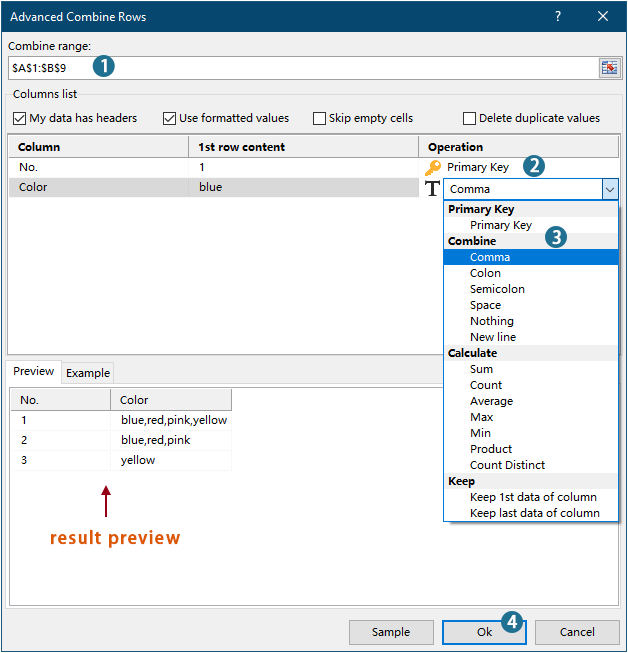
วิธีการที่อธิบายไว้ข้างต้นจำเป็นต้องสร้างคอลัมน์ตัวช่วยสองคอลัมน์และเกี่ยวข้องกับหลายขั้นตอน ซึ่งอาจไม่สะดวก หากคุณกำลังมองหาวิธีที่ง่ายกว่านี้ ให้พิจารณาใช้ แถวรวมขั้นสูง เครื่องมือจาก Kutools สำหรับ Excel. ด้วยการคลิกเพียงไม่กี่ครั้ง ยูทิลิตีนี้ช่วยให้คุณสามารถเชื่อมเซลล์เข้าด้วยกันโดยใช้ตัวคั่นเฉพาะ ทำให้กระบวนการรวดเร็วและไม่ยุ่งยาก

ปลาย: ก่อนใช้เครื่องมือนี้ โปรดติดตั้ง Kutools สำหรับ Excel ประการแรก ไปดาวน์โหลดฟรีเลย.

1 คลิก Kutools > ผสานและแยก > แถวรวมขั้นสูง เพื่อเปิดใช้งานคุณสมบัตินี้
2 ใน แถวรวมขั้นสูง กล่องโต้ตอบ คุณเพียงแค่ต้อง:
  • เลือกช่วงที่คุณต้องการเชื่อม
  • ตั้งค่าคอลัมน์ด้วยค่าเดียวกับ คีย์หลัก คอลัมน์.
  • ระบุตัวคั่นเพื่อรวมเซลล์
  • คลิก OK.

ผล

หมายเหตุ:

เชื่อมต่อเซลล์ถ้าค่าเดียวกันกับรหัส VBA

คุณยังสามารถใช้รหัส VBA เพื่อเชื่อมเซลล์ในคอลัมน์ ถ้าค่าเดียวกันอยู่ในคอลัมน์อื่น

1 กด อื่น ๆ + F11 คีย์เพื่อเปิด แอปพลิเคชัน Microsoft Visual Basic หน้าต่าง

2 ใน แอปพลิเคชัน Microsoft Visual Basic หน้าต่างคลิก สิ่งที่ใส่เข้าไป > โมดูล. จากนั้นคัดลอกและวางโค้ดด้านล่างลงในไฟล์ โมดูล หน้าต่าง

รหัส VBA: เชื่อมต่อเซลล์หากมีค่าเท่ากัน

Sub ConcatenateCellsIfSameValues()
	Dim xCol As New Collection
	Dim xSrc As Variant
	Dim xRes() As Variant
	Dim I As Long
	Dim J As Long
	Dim xRg As Range
	xSrc    = Range("A1", Cells(Rows.Count, "A").End(xlUp)).Resize(, 2)
	Set xRg = Range("D1")
	On Error Resume Next
	For I = 2 To UBound(xSrc)
		xCol.Add xSrc(I, 1), TypeName(xSrc(I, 1)) & CStr(xSrc(I, 1))
	Next I
	On Error GoTo 0
	ReDim xRes(1 To xCol.Count + 1, 1 To 2)
	xRes(1, 1) = "No"
	xRes(1, 2) = "Combined Color"
	For I = 1 To xCol.Count
		xRes(I + 1, 1) = xCol(I)
		For J = 2 To UBound(xSrc)
			If xSrc(J, 1) = xRes(I + 1, 1) Then
				xRes(I + 1, 2) = xRes(I + 1, 2) & ", " & xSrc(J, 2)
			End If
		Next J
		xRes(I + 1, 2) = Mid(xRes(I + 1, 2), 2)
	Next I
	Set xRg = xRg.Resize(UBound(xRes, 1), UBound(xRes, 2))
	xRg.NumberFormat = "@"
	xRg = xRes
	xRg.EntireColumn.AutoFit
End Sub

หมายเหตุ / รายละเอียดเพิ่มเติม:

1. D1 ในสาย ตั้งค่า xRg = ช่วง ("D1") หมายความว่าผลลัพธ์จะถูกวางไว้โดยเริ่มจากเซลล์ D1
2 'ไม่"และ "สีผสม" ในสาย xRes (1, 1) = "ไม่ใช่" และ xRes (1, 2) = "สีรวม" เป็นส่วนหัวของคอลัมน์ที่เลือก 

3 กด F5 คีย์เพื่อรันโค้ดจากนั้นคุณจะได้ผลลัพธ์ที่ต่อกันในช่วงที่ระบุ


เชื่อมต่อเซลล์ได้อย่างง่ายดายหากค่าเดียวกันกับ Kutools for Excel

สุดยอดเครื่องมือเพิ่มผลผลิตในสำนักงาน

🤖 Kutools AI ผู้ช่วย: ปฏิวัติการวิเคราะห์ข้อมูลโดยยึดตาม: การดำเนินการที่ชาญฉลาด   |  สร้างรหัส  |  สร้างสูตรที่กำหนดเอง  |  วิเคราะห์ข้อมูลและสร้างแผนภูมิ  |  เรียกใช้ฟังก์ชัน Kutools...
คุณสมบัติยอดนิยม: ค้นหา เน้น หรือระบุรายการที่ซ้ำกัน   |  ลบแถวว่าง   |  รวมคอลัมน์หรือเซลล์โดยไม่สูญเสียข้อมูล   |   รอบโดยไม่มีสูตร ...
การค้นหาขั้นสูง: VLookup หลายเกณฑ์    VLookup หลายค่า  |   VLookup ข้ามหลายแผ่น   |   การค้นหาที่ไม่ชัดเจน ....
รายการแบบเลื่อนลงขั้นสูง: สร้างรายการแบบหล่นลงอย่างรวดเร็ว   |  รายการแบบหล่นลงขึ้นอยู่กับ   |  เลือกหลายรายการแบบหล่นลง ....
ผู้จัดการคอลัมน์: เพิ่มจำนวนคอลัมน์เฉพาะ  |  ย้ายคอลัมน์  |  สลับสถานะการมองเห็นของคอลัมน์ที่ซ่อนอยู่  |  เปรียบเทียบช่วงและคอลัมน์ ...
คุณสมบัติเด่น: กริดโฟกัส   |  มุมมองการออกแบบ   |   บาร์สูตรใหญ่    สมุดงานและตัวจัดการชีต   |  ห้องสมุดทรัพยากร (ข้อความอัตโนมัติ)   |  เลือกวันที่   |  รวมแผ่นงาน   |  เข้ารหัส/ถอดรหัสเซลล์    ส่งอีเมลตามรายการ   |  ซุปเปอร์ฟิลเตอร์   |   ตัวกรองพิเศษ (กรองตัวหนา/ตัวเอียง/ขีดทับ...) ...
ชุดเครื่องมือ 15 อันดับแรก12 ข้อความ เครื่องมือ (เพิ่มข้อความ, ลบอักขระ, ... )   |   50 + แผนภูมิ ประเภท (แผนภูมิ Gantt, ... )   |   40+ ใช้งานได้จริง สูตร (คำนวณอายุตามวันเกิด, ... )   |   19 การแทรก เครื่องมือ (ใส่ QR Code, แทรกรูปภาพจากเส้นทาง, ... )   |   12 การแปลง เครื่องมือ (ตัวเลขเป็นคำ, การแปลงสกุลเงิน, ... )   |   7 ผสานและแยก เครื่องมือ (แถวรวมขั้นสูง, แยกเซลล์, ... )   |   ... และอื่น ๆ

เพิ่มพูนทักษะ Excel ของคุณด้วย Kutools สำหรับ Excel และสัมผัสประสิทธิภาพอย่างที่ไม่เคยมีมาก่อน Kutools สำหรับ Excel เสนอคุณสมบัติขั้นสูงมากกว่า 300 รายการเพื่อเพิ่มประสิทธิภาพและประหยัดเวลา  คลิกที่นี่เพื่อรับคุณสมบัติที่คุณต้องการมากที่สุด...

รายละเอียด


แท็บ Office นำอินเทอร์เฟซแบบแท็บมาที่ Office และทำให้งานของคุณง่ายขึ้นมาก

  • เปิดใช้งานการแก้ไขและอ่านแบบแท็บใน Word, Excel, PowerPoint, ผู้จัดพิมพ์, Access, Visio และโครงการ
  • เปิดและสร้างเอกสารหลายรายการในแท็บใหม่ของหน้าต่างเดียวกันแทนที่จะเป็นในหน้าต่างใหม่
  • เพิ่มประสิทธิภาพการทำงานของคุณ 50% และลดการคลิกเมาส์หลายร้อยครั้งให้คุณทุกวัน!
Comments (23)
No ratings yet. Be the first to rate!
This comment was minimized by the moderator on the site
thank you very much, the VBA code works very well but I have a question that I can't solve.

NO Color
1 red
1 blue
1 red
1 yellow
2 red
2 yellow


in this case, in column B we have some duplicate colors related to the same number. How can I have an output that only return the values once?

I would like an output like this

NO Color
1 red, blue, yellow
2 red, yellow
This comment was minimized by the moderator on the site
Hi

The second method described in the post can help you solve this problem. After following the steps to specify the settings, checking the Delect Duplicate Values option will delete all duplicates in the combined results.
https://www.extendoffice.com/images/stories/comments/comment-picture-zxm/concatenate.png
This comment was minimized by the moderator on the site
Thank you so much for this formula! It saved hours of investigation! Fantastic work :)
This comment was minimized by the moderator on the site
Hi Crystal,

Thanks for your reply. I'll have to put my thinking hat on again...
Thank you
This comment was minimized by the moderator on the site
Hello, the macro above works great! Thank you. Is it anyway possible (I tried, but not successful) to amend it to concatenate column B (description) based on duplicates in column A (HS code) but also taking column C (origin) in the combination?
So description texts concatenate per HS code per origin.
Also column D(quantity) and column E(value) must be summed per HS code and origin.

A B C D E
HS CODE DESCRIPTION ORIGIN QUANTITY VALUE
5407420000 TWEED CN 10 € 150,00
5407420000 COTTON CN 15 € 250,00
5407420000 POLYESTER TW 5 € 130,00
5407420000 ORGANIC COTTON US 18 € 450,00
5407420000 COTTON US 23 € 780,00
5407420000 VELVET DELUXE CN 20 € 380,00
5407420000 COTTON CN 10 € 120,00
5806310000 TWEED JP 15 € 35,00
5806310000 POLYESTER AU 20 € 78,00
5806310000 TWEED AU 25 € 254,00
5806310000 POLYESTER SG 130 € 888,00
5806310000 COTTON EU 120 € 945,00
5806310000 COTTON FABRIC EU 10 € 80,00


Result shopuld be:

5407420000 TWEED, COTTON, VELVET DULUXE, COTTON, CN 55 € 900,00
5407420000 POLYESTER TW 5 € 130,00
5407420000 ORGANIC COTTON, COTTON US 41 € 1230,00
5806310000 TWEED JP 15 € 35,00
5806310000 POLYESTER, TWEED AU 45 € 332,00
5806310000 POLYESTER SG 130 € 888,00
5806310000 COTTON, COTTON FABRIC EU 130 € 1025,00

I hope this possible, thank you!
This comment was minimized by the moderator on the site
Hi Ivar,

Thank you for your comment. I am not able to solve this problem with VBA code yet. Sorry for that.
You can try if the last method can help.
This comment was minimized by the moderator on the site
Hello, how would the VBA code be adjusted if I want to combine cells in column M based on the duplicates in column A?
This comment was minimized by the moderator on the site
Hi Kristin,To combine cells in column M based on the duplicates in column A, try the VBA below.In the code,  O1 is the first cell to output the results; M is the column you will combine based on the duplicates in column A; A1 and A represent the first cell and the column where the duplicates locate; No and Combine color is the header of the columns after concatenating. You can change these variables as needed.<div data-tag="code">Sub ConcatenateCellsIfSameValues()
'Updated by Extendoffice 20211105
Dim xCol As New Collection
Dim xSrc As Variant
Dim xSrcValue As Variant
Dim xRes() As Variant
Dim I As Long
Dim J As Long
Dim xRg As Range
Dim xResultAddress As String
Dim xMergeAddress As String
Dim xUp As Integer

xResultAddress = "O1" 'The cell to output the results
xMergeAddress = "M" 'The column you will combine based on the duplicates in column A

xSrc = Range("A1", Cells(Rows.Count, "A").End(xlUp)).Resize(, 1)
xUp = Range("A1", Cells(Rows.Count, "A").End(xlUp)).Rows.Count
xSrcValue = Range(xMergeAddress & "1:" & xMergeAddress & xUp)

Set xRg = Range(xResultAddress)
On Error Resume Next
For I = 2 To UBound(xSrc)
xCol.Add xSrc(I, 1), TypeName(xSrc(I, 1)) & CStr(xSrc(I, 1))
Next I

On Error GoTo 0
ReDim xRes(1 To xCol.Count + 1, 1 To 2)
xRes(1, 1) = "No"
xRes(1, 2) = "Combined Color"
For I = 1 To xCol.Count
xRes(I + 1, 1) = xCol(I)
For J = 2 To UBound(xSrc)
If xSrc(J, 1) = xRes(I + 1, 1) Then
xRes(I + 1, 2) = xRes(I + 1, 2) & ", " & xSrcValue(J, 1)
End If
Next J
xRes(I + 1, 2) = Mid(xRes(I + 1, 2), 2)
Next I
Set xRg = xRg.Resize(UBound(xRes, 1), UBound(xRes, 2))
xRg.NumberFormat = "@"
xRg = xRes
xRg.EntireColumn.AutoFit
End Sub
This comment was minimized by the moderator on the site
I just wanted to thank you. It wasn't exactly what I wanted but man did it help me figure out what to do.

I have a table where the person's name was in column A, dates in column B and the names of tools they use in the headers of columns C:G . In each column there is a "Y" if they used that tool on that date and blank if they did not. (FYI: the same person can be listed more than once and may have used the same tool more than once) On a separate (summary) page I wanted to list all tools each person used within a date period, only listing each tool they used once, in the same cell. On this page, the person's name was in column A, Types of tools used in column B and the helper columns were in column G:K. Here's what I got:
The first helper column (G2):
=IF(COUNTIFS(Table7[Person's Name],A2,Table7[Screw Driver],"Y",Table7[Date],">="&1/1/20,Table7[Date],"<="&3/31/20),"Screw Driver","")
In the last helper column (K2):
=IF(COUNTIFS(Table7[Person's Name],A2,Table7[Hammer],"Y",Table7[Date],">="&1/1/20,Table7[Date],"<="&3/31/20),IF(J2="","Hammer",J2&"/"&"Hammer"),J2)

In B2 I just entered =K2

Thanks again and I hope this helps someone. EZPD
This comment was minimized by the moderator on the site
Hi, first of all thanks for creating this resource. I have been trying to figure this out for a couple of hours and I'm stuck. I'm using your 'concatenate cells if same value' but my script is looking at column "D" instead of "A. I can't figure out how to get it to use a different column for the data besides the one right next to it. In my cases I want it to look at column "D" to see if the value is the same and if so, it will grab the data from column "H" and put that data from column "H' into a cell in column "J". How do I switch this to use column "H" for the data? Thx


Sub ConcatenateCellsIfSameValues()
Dim xCol As New Collection
Dim xSrc As Variant
Dim xRes() As Variant
Dim I As Long
Dim J As Long
Dim xRg As Range
xSrc = Range("D1", Cells(Rows.Count, "D").End(xlUp)).Resize(, 2)
Set xRg = Range("J1")
On Error Resume Next
For I = 2 To UBound(xSrc)
xCol.Add xSrc(I, 1), TypeName(xSrc(I, 1)) & CStr(xSrc(I, 1))
Next I
On Error GoTo 0
ReDim xRes(1 To xCol.Count + 1, 1 To 2)
xRes(1, 1) = "No"
xRes(1, 2) = "Products"
For I = 1 To xCol.Count
xRes(I + 1, 1) = xCol(I)
For J = 2 To UBound(xSrc)
If xSrc(J, 1) = xRes(I + 1, 1) Then
xRes(I + 1, 2) = xRes(I + 1, 2) & vbCrLf & xSrc(J, 2)
End If
Next J
xRes(I + 1, 2) = Mid(xRes(I + 1, 2), 2)
Next I
Set xRg = xRg.Resize(UBound(xRes, 1), UBound(xRes, 2))
xRg.NumberFormat = "@"
xRg = xRes
xRg.EntireColumn.AutoFit
End Sub
This comment was minimized by the moderator on the site
"I can't figure out how to get it to use a different column for the data besides the one right next to it. In my cases I want it to look at column 'D' to see if the value is the same and if so, it will grab the data from column 'H' and put that data from column 'H' into a cell in column 'J'."

Did you ever figure this out?
This comment was minimized by the moderator on the site
Hi,

looks like 2 of your formulas are wrong :

=IF(A2<>A3,CONCATENATE(A2,",""",C2,""""),""). You need to change "A2" to "D1". As you'll want to add the string to the previous cell.

same goes for this formula :

=IF(A2<>A1,B2,C1 & "," & B2) : Change C1 to D1.


kind regards


Harry
This comment was minimized by the moderator on the site
I use this VBA for lots of my spreadsheets and its great. But the spreadsheets have become very large 50k+ rows and it doesnt seem to be working any more. If I use it on 1000 rows it works fine but large sets of data it cant seem to cope with. No errors just no results. Any help would be appreciated.
This comment was minimized by the moderator on the site
Hi James,
I tested the code as you mentioned, but it still works well in my case even I set the rows to 1000+.
This comment was minimized by the moderator on the site
Using the VBA macro and getting great results, I have tried tweaking it slightly for my needs but cant get it to work so I hope you can help.

Which bit do I change to make it concat a specific column, not the one directly to the right of the xSrc = Range?

Thanks for your great work!
This comment was minimized by the moderator on the site
Or as a better option, if you had 3 columns instead of 2 and found duplicates in column A (like your example) can you concat column B into a cell and column C into a seperate cell? So if you had columns of Number, Colour, Age, could you concat colour and age into different columns upon finding duplicates in Number? Hope that makes sense!
There are no comments posted here yet
Load More
Please leave your comments in English
Posting as Guest
×
Rate this post:
0   Characters
Suggested Locations