ไปยังเนื้อหาหลัก

วิธีจัดเรียงข้อมูลตัวอักษรและตัวเลขใน Excel

หากคุณมีรายการข้อมูลที่ผสมกับทั้งตัวเลขและสตริงข้อความเมื่อคุณเรียงลำดับข้อมูลคอลัมน์นี้ตามปกติใน Excel ตัวเลขทั้งหมดจะถูกจัดเรียงไว้ด้านบนและสตริงข้อความผสมที่ด้านล่าง แต่ผลลัพธ์ที่คุณต้องการเช่นภาพหน้าจอสุดท้ายที่แสดง บทความนี้จะให้วิธีการที่มีประโยชน์ซึ่งคุณสามารถใช้เพื่อจัดเรียงข้อมูลที่เป็นตัวอักษรและตัวเลขใน Excel เพื่อให้คุณได้ผลลัพธ์ที่ต้องการ

จัดเรียงข้อมูลตัวอักษรและตัวเลขด้วยคอลัมน์ตัวช่วยสูตร

ข้อมูลต้นฉบับ   โดยปกติจะเรียงลำดับผลลัพธ์   ผลการจัดเรียงที่คุณต้องการ
doc เรียงลำดับตัวเลขและตัวอักษร 1 2 doc เรียงลำดับตัวเลขและตัวอักษร 2 2 doc เรียงลำดับตัวเลขและตัวอักษร 3

ลูกศรสีฟ้าฟองขวา จัดเรียงข้อมูลตัวอักษรและตัวเลขด้วยคอลัมน์ตัวช่วยสูตร

ใน Excel คุณสามารถสร้างคอลัมน์ตัวช่วยสูตรแล้วจัดเรียงข้อมูลตามคอลัมน์ใหม่นี้โปรดทำตามขั้นตอนต่อไปนี้:

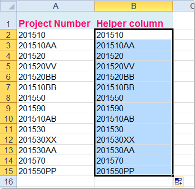
1. ใส่สูตรนี้ = ข้อความ (A2, "###") ลงในเซลล์ว่างนอกเหนือจากข้อมูลของคุณเช่น B2 ดูภาพหน้าจอ:

doc เรียงลำดับตัวเลขและตัวอักษร 4

2. จากนั้นลากที่จับเติมลงไปที่เซลล์ที่คุณต้องการใช้สูตรนี้ดูภาพหน้าจอ:

doc เรียงลำดับตัวเลขและตัวอักษร 5

3. จากนั้นจัดเรียงข้อมูลตามคอลัมน์ใหม่นี้เลือกคอลัมน์ผู้ช่วยเหลือที่คุณสร้างขึ้นจากนั้นคลิก ข้อมูล > ประเภทและในกล่องพรอมต์ที่โผล่ขึ้นมาให้เลือก ขยายส่วนที่เลือกดูภาพหน้าจอ:

doc เรียงลำดับตัวเลขและตัวอักษร 6 2 doc เรียงลำดับตัวเลขและตัวอักษร 7

4. และคลิก ประเภท เพื่อเปิด ประเภท ไดอะล็อกภายใต้ คอลัมน์ ส่วนเลือก คอลัมน์ตัวช่วย ชื่อที่คุณต้องการจัดเรียงและใช้ ความคุ้มค่า ภายใต้ จัดเรียงบน จากนั้นเลือกลำดับการจัดเรียงตามที่คุณต้องการดูภาพหน้าจอ:

doc เรียงลำดับตัวเลขและตัวอักษร 8

5. จากนั้นคลิก OKในกล่องโต้ตอบคำเตือนการจัดเรียงที่โผล่ออกมาโปรดเลือก จัดเรียงตัวเลขและตัวเลขที่จัดเก็บเป็นข้อความแยกกันดูภาพหน้าจอ:

doc เรียงลำดับตัวเลขและตัวอักษร 9

6. จากนั้นคลิก OK คุณจะเห็นว่าข้อมูลได้รับการจัดเรียงตามความต้องการของคุณ

doc เรียงลำดับตัวเลขและตัวอักษร 10

7. ในที่สุดคุณสามารถลบเนื้อหาของคอลัมน์ผู้ช่วยเหลือได้ตามที่คุณต้องการ

สุดยอดเครื่องมือเพิ่มผลผลิตในสำนักงาน

🤖 Kutools AI ผู้ช่วย: ปฏิวัติการวิเคราะห์ข้อมูลโดยยึดตาม: การดำเนินการที่ชาญฉลาด   |  สร้างรหัส  |  สร้างสูตรที่กำหนดเอง  |  วิเคราะห์ข้อมูลและสร้างแผนภูมิ  |  เรียกใช้ฟังก์ชัน Kutools...
คุณสมบัติยอดนิยม: ค้นหา เน้น หรือระบุรายการที่ซ้ำกัน   |  ลบแถวว่าง   |  รวมคอลัมน์หรือเซลล์โดยไม่สูญเสียข้อมูล   |   รอบโดยไม่มีสูตร ...
การค้นหาขั้นสูง: VLookup หลายเกณฑ์    VLookup หลายค่า  |   VLookup ข้ามหลายแผ่น   |   การค้นหาที่ไม่ชัดเจน ....
รายการแบบเลื่อนลงขั้นสูง: สร้างรายการแบบหล่นลงอย่างรวดเร็ว   |  รายการแบบหล่นลงขึ้นอยู่กับ   |  เลือกหลายรายการแบบหล่นลง ....
ผู้จัดการคอลัมน์: เพิ่มจำนวนคอลัมน์เฉพาะ  |  ย้ายคอลัมน์  |  สลับสถานะการมองเห็นของคอลัมน์ที่ซ่อนอยู่  |  เปรียบเทียบช่วงและคอลัมน์ ...
คุณสมบัติเด่น: กริดโฟกัส   |  มุมมองการออกแบบ   |   บาร์สูตรใหญ่    สมุดงานและตัวจัดการชีต   |  ห้องสมุดทรัพยากร (ข้อความอัตโนมัติ)   |  เลือกวันที่   |  รวมแผ่นงาน   |  เข้ารหัส/ถอดรหัสเซลล์    ส่งอีเมลตามรายการ   |  ซุปเปอร์ฟิลเตอร์   |   ตัวกรองพิเศษ (กรองตัวหนา/ตัวเอียง/ขีดทับ...) ...
ชุดเครื่องมือ 15 อันดับแรก12 ข้อความ เครื่องมือ (เพิ่มข้อความ, ลบอักขระ, ... )   |   50 + แผนภูมิ ประเภท (แผนภูมิ Gantt, ... )   |   40+ ใช้งานได้จริง สูตร (คำนวณอายุตามวันเกิด, ... )   |   19 การแทรก เครื่องมือ (ใส่ QR Code, แทรกรูปภาพจากเส้นทาง, ... )   |   12 การแปลง เครื่องมือ (ตัวเลขเป็นคำ, การแปลงสกุลเงิน, ... )   |   7 ผสานและแยก เครื่องมือ (แถวรวมขั้นสูง, แยกเซลล์, ... )   |   ... และอื่น ๆ

เพิ่มพูนทักษะ Excel ของคุณด้วย Kutools สำหรับ Excel และสัมผัสประสิทธิภาพอย่างที่ไม่เคยมีมาก่อน Kutools สำหรับ Excel เสนอคุณสมบัติขั้นสูงมากกว่า 300 รายการเพื่อเพิ่มประสิทธิภาพและประหยัดเวลา  คลิกที่นี่เพื่อรับคุณสมบัติที่คุณต้องการมากที่สุด...

รายละเอียด


แท็บ Office นำอินเทอร์เฟซแบบแท็บมาที่ Office และทำให้งานของคุณง่ายขึ้นมาก

  • เปิดใช้งานการแก้ไขและอ่านแบบแท็บใน Word, Excel, PowerPoint, ผู้จัดพิมพ์, Access, Visio และโครงการ
  • เปิดและสร้างเอกสารหลายรายการในแท็บใหม่ของหน้าต่างเดียวกันแทนที่จะเป็นในหน้าต่างใหม่
  • เพิ่มประสิทธิภาพการทำงานของคุณ 50% และลดการคลิกเมาส์หลายร้อยครั้งให้คุณทุกวัน!
Comments (10)
No ratings yet. Be the first to rate!
This comment was minimized by the moderator on the site
The stock symbol for TrueCar Inc is "TRUE". When I sort the column containing the stock symbols, TRUE falls out of place at the end of the list. The cell is formatted as text. I am assuming that it is because "TRUE" has special meaning in Excel. Right now I am removing the "E", sorting the column so the row falls in the right place and then adding the E after the sort. Any ideas on a better approach?  
This comment was minimized by the moderator on the site
Hi, I have a similar sorting requirement, but with a unique problem ....
I have a range of Stock data which I need to sort in Category order.
The Range includes prices and one column has formulas.
The Category numbers range from 1 1a 1b etc to 32e.
I have continuously tried using a helper column with the formula =TEXT(K3,"###") - with K3 being the first Row in the Category column.
I select the helper column (N) and click Data - Sort - Expand the selection, but get no further as the "expansion" always selects from Row 40 - even if I select just a few rows in the helper column.
Why is this, and how can I sort my data correctly ?
Looking forward to a solution ....
Thanks.
Patrick.
This comment was minimized by the moderator on the site
Thanks for the tip on using a "helper column", but here's my question:

Is there a way to get the "related " columns to "tag along" with the sort precipitated by the helper column?

For example, column A contains a mixed-string product code that I can now sort into sequence using the "helper column" technique but, attached to that same product code are product descriptions, dimensions and other characteristics (some of which are also mixed-string in nature) in several other columns, and I need those to follow the "helper column" sort.

Any suggestions?

Much appreciated!

Lorne
This comment was minimized by the moderator on the site
I only see 1 method. Top of the article mentions that we will see 2 methods.
This comment was minimized by the moderator on the site
Hello, val,
Thank you for your comment, it is my mistake, I have deleted the second method from this article, and now, I have updated the article.

Thank you once more!
This comment was minimized by the moderator on the site
Trying to sort Alphanumeric with text. It is a fairly large list but below is an example. I can't strip the off the letter in a different column and sort by that because I have matching numbers that should come before them. I also can't really add a column to sort by and then hide that column - or delete it because I am constantly sorting the data. Any ideas? Will there be some formula? My current list: ---- What I want it to look like: 1 ---- 1 2 ---- 2 3 ---- 3 4 ---- 4 A1 ---- A1 A10 ---- A2 A100 ---- A3 A2 ---- A4 A20 ---- A5 A200 ---- A6 A3 ---- A7 A4 ---- A8 A5 ---- A9 A6 ---- A10 A60 ---- A20 A7 ---- A60 A8 ---- A100 A9 ---- A200
This comment was minimized by the moderator on the site
The easiest way I can think is to split the column into the Alpha part ("A") and the numeric part ("1") and then sort first by alpha then by numeric.
Your original 1,2,3,4 would need to stay in the alpha column to sort properly .

N.B. this might be a bit more difficult to achieve when the alpha part (the "A") is not a consistent length in your data. But definitely still possible.
This comment was minimized by the moderator on the site
I am running in the same problem. I have 1200 part numbers that I need to sort the way it's shown above but excel will put V15 after V1 if V14 is absent. I need V14 to appear after V9 or V8, where ever the part number ends.
This comment was minimized by the moderator on the site
Trying to sort Alphanumeric with text. It is a fairly large list but below is an example. I can't strip the off the letter in a different column and sort by that because I have matching numbers that should come before them. I also can't really add a column to sort by and then hide that column - or delete it because I am constantly sorting the data. Any ideas? My current list: ---- What I want it to look like: 1 ---- 1 2 ---- 2 3 ---- 3 4 ---- 4 A1 ---- A1 A10 ---- A2 A100 ---- A3 A2 ---- A4 A20 ---- A5 A200 ---- A6 A3 ---- A7 A4 ---- A8 A5 ---- A9 A6 ---- A10 A60 ---- A20 A7 ---- A60 A8 ---- A100 A9 ---- A200
This comment was minimized by the moderator on the site
When I do this, the column sorts by individual character and I don't get the right order. For instance, if I have the following data: A1: 1 A2: 2 A3: 1a1 A4: 12 A5: 1a2 I want them to be sorted like this: A1: 1 A2: 1a1 A3: 1a2 A4: 2 A5: 12 Just sorting the column normally I end up with this: A1: 1 A2: 2 A3: 12 A4: 1a1 A5: 1a2 Where the numbers are sorted correctly and then the alphanumeric values are sorted correctly, but the two are not sorted together. When I use the method in the article, I end up with this: A1: 1 A2: 12 A3: 1a1 A4: 1a2 A5: 2 Where the numeric and alphanumeric data are sorted together but incorrectly (12 should come after 2). Why is this happening?
There are no comments posted here yet
Please leave your comments in English
Posting as Guest
×
Rate this post:
0   Characters
Suggested Locations