ไปยังเนื้อหาหลัก

วิธี VLOOKUP และส่งคืนค่าที่เกี่ยวข้องหลายค่าในแนวนอนใน Excel

doc-vlookup- แนวนอน -1
ตามค่าเริ่มต้นฟังก์ชัน VLOOKUP สามารถส่งคืนค่าที่เกี่ยวข้องได้หลายค่าในระดับแนวตั้งใน Excel ในบางกรณีคุณอาจต้องการส่งคืนค่าหลายค่าในระดับแนวนอนดังภาพด้านล่างที่แสดง ที่นี่ฉันจะบอกสูตรที่สามารถแก้ปัญหานี้ได้
VLOOKUP และส่งคืนค่าหลายค่าในแนวนอน

ลูกศรสีฟ้าฟองขวา VLOOKUP และส่งคืนค่าหลายค่าในแนวนอน

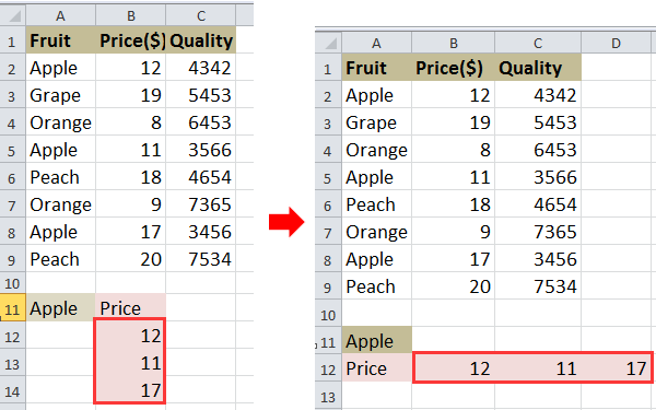
ตัวอย่างเช่นคุณมีช่วงข้อมูลตามภาพด้านล่างที่แสดงและคุณต้องการ VLOOKUP ราคาของ Apple
doc-vlookup- แนวนอน -2

1. เลือกเซลล์และพิมพ์สูตรนี้ =INDEX($B$2:$B$9, SMALL(IF($A$11=$A$2:$A$9, ROW($A$2:$A$9)-ROW($A$2)+1), COLUMN(A1))) เข้าไปแล้วกด Shift + Ctrl + Enter แล้วลากที่จับการป้อนอัตโนมัติไปทางขวาเพื่อใช้สูตรนี้จนถึง # หนึ่งเดียว! ปรากฏขึ้น ดูภาพหน้าจอ:
doc-vlookup- แนวนอน -3

2. จากนั้นลบ #NUM! ดูภาพหน้าจอ:
doc-vlookup- แนวนอน -4

เคล็ดลับ: ในสูตรข้างต้น B2: B9 คือช่วงคอลัมน์ที่คุณต้องการส่งคืนค่าใน A2: A9 คือช่วงคอลัมน์ที่ค่าการค้นหาอยู่ A11 คือค่าการค้นหา A1 เป็นเซลล์แรกของช่วงข้อมูลของคุณ A2 คือเซลล์แรกของช่วงคอลัมน์ที่คุณค้นหาค่า

หากคุณต้องการส่งคืนค่าหลายค่าในแนวตั้งคุณสามารถอ่านบทความนี้ วิธีการค้นหาค่าส่งคืนค่าที่เกี่ยวข้องหลายค่าใน Excel


รวมหลายแผ่นงาน / สมุดงานเป็นแผ่นงานเดียวหรือสมุดงาน

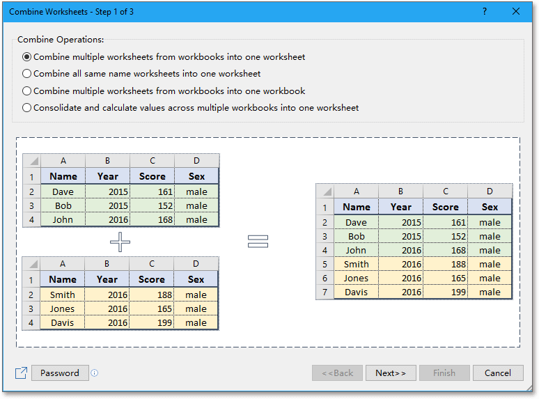
ในการรวมแผ่นงานหลายแผ่นหรือสมุดงานเป็นแผ่นงานเดียวหรือสมุดงานอาจเป็นเรื่องที่น่าสนใจใน Excel แต่ด้วยไฟล์ รวมกัน ฟังก์ชันใน Kutools สำหรับ Excel คุณสามารถรวมแผ่นงาน / สมุดงานหลายสิบแผ่นไว้ในแผ่นงานหรือสมุดงานเดียวได้นอกจากนี้คุณยังสามารถรวมแผ่นงานเข้าด้วยกันโดยคลิกเพียงไม่กี่ครั้งเท่านั้น  คลิกเพื่อทดลองใช้งานฟรี 30 วันเต็มรูปแบบ!
รวมแผ่น
 
Kutools for Excel: มีโปรแกรมเสริม Excel ที่มีประโยชน์มากกว่า 300 รายการให้ทดลองใช้ฟรีโดยไม่มีข้อ จำกัด ใน 30 วัน

สุดยอดเครื่องมือเพิ่มผลผลิตในสำนักงาน

🤖 Kutools AI ผู้ช่วย: ปฏิวัติการวิเคราะห์ข้อมูลโดยยึดตาม: การดำเนินการที่ชาญฉลาด   |  สร้างรหัส  |  สร้างสูตรที่กำหนดเอง  |  วิเคราะห์ข้อมูลและสร้างแผนภูมิ  |  เรียกใช้ฟังก์ชัน Kutools...
คุณสมบัติยอดนิยม: ค้นหา เน้น หรือระบุรายการที่ซ้ำกัน   |  ลบแถวว่าง   |  รวมคอลัมน์หรือเซลล์โดยไม่สูญเสียข้อมูล   |   รอบโดยไม่มีสูตร ...
การค้นหาขั้นสูง: VLookup หลายเกณฑ์    VLookup หลายค่า  |   VLookup ข้ามหลายแผ่น   |   การค้นหาที่ไม่ชัดเจน ....
รายการแบบเลื่อนลงขั้นสูง: สร้างรายการแบบหล่นลงอย่างรวดเร็ว   |  รายการแบบหล่นลงขึ้นอยู่กับ   |  เลือกหลายรายการแบบหล่นลง ....
ผู้จัดการคอลัมน์: เพิ่มจำนวนคอลัมน์เฉพาะ  |  ย้ายคอลัมน์  |  สลับสถานะการมองเห็นของคอลัมน์ที่ซ่อนอยู่  |  เปรียบเทียบช่วงและคอลัมน์ ...
คุณสมบัติเด่น: กริดโฟกัส   |  มุมมองการออกแบบ   |   บาร์สูตรใหญ่    สมุดงานและตัวจัดการชีต   |  ห้องสมุดทรัพยากร (ข้อความอัตโนมัติ)   |  เลือกวันที่   |  รวมแผ่นงาน   |  เข้ารหัส/ถอดรหัสเซลล์    ส่งอีเมลตามรายการ   |  ซุปเปอร์ฟิลเตอร์   |   ตัวกรองพิเศษ (กรองตัวหนา/ตัวเอียง/ขีดทับ...) ...
ชุดเครื่องมือ 15 อันดับแรก12 ข้อความ เครื่องมือ (เพิ่มข้อความ, ลบอักขระ, ... )   |   50 + แผนภูมิ ประเภท (แผนภูมิ Gantt, ... )   |   40+ ใช้งานได้จริง สูตร (คำนวณอายุตามวันเกิด, ... )   |   19 การแทรก เครื่องมือ (ใส่ QR Code, แทรกรูปภาพจากเส้นทาง, ... )   |   12 การแปลง เครื่องมือ (ตัวเลขเป็นคำ, การแปลงสกุลเงิน, ... )   |   7 ผสานและแยก เครื่องมือ (แถวรวมขั้นสูง, แยกเซลล์, ... )   |   ... และอื่น ๆ

เพิ่มพูนทักษะ Excel ของคุณด้วย Kutools สำหรับ Excel และสัมผัสประสิทธิภาพอย่างที่ไม่เคยมีมาก่อน Kutools สำหรับ Excel เสนอคุณสมบัติขั้นสูงมากกว่า 300 รายการเพื่อเพิ่มประสิทธิภาพและประหยัดเวลา  คลิกที่นี่เพื่อรับคุณสมบัติที่คุณต้องการมากที่สุด...

รายละเอียด


แท็บ Office นำอินเทอร์เฟซแบบแท็บมาที่ Office และทำให้งานของคุณง่ายขึ้นมาก

  • เปิดใช้งานการแก้ไขและอ่านแบบแท็บใน Word, Excel, PowerPoint, ผู้จัดพิมพ์, Access, Visio และโครงการ
  • เปิดและสร้างเอกสารหลายรายการในแท็บใหม่ของหน้าต่างเดียวกันแทนที่จะเป็นในหน้าต่างใหม่
  • เพิ่มประสิทธิภาพการทำงานของคุณ 50% และลดการคลิกเมาส์หลายร้อยครั้งให้คุณทุกวัน!
Comments (20)
No ratings yet. Be the first to rate!
This comment was minimized by the moderator on the site
This article says this uses VLOOKUP, but it uses INDEX... which does not help me. I need a solution for multiple values using VLOOKUP or XLOOKUP in tables.
This comment was minimized by the moderator on the site
you can use TEXTSPLIT function followed by TEXTJOIN FUNCTION in excel 365
This comment was minimized by the moderator on the site
For anyone experiencing issues in a big data range, ensure you dont have any cells existent with "#N/A" or it will break it. Simple error but can be overlooked.
This comment was minimized by the moderator on the site
Hello, I want to use keyword instead of specific text or value here for multiple return values, can you please share code formula for same.
This comment was minimized by the moderator on the site
Hello - This formula worked perfectly - thank you! However, I want to apply it to a long list of lookup values. When I copy and paste the formula it obviously returns the same results as the first lookup value so I removed the $'s from $A$11, but that changes the result to something incorrect. How can I quickly apply this same formula for a long list of lookup values?

Thank you!

M
This comment was minimized by the moderator on the site
Bonjour,

J'ai retransposé mon problème exactement dans les mêmes positions de colonne que l'exemple et j’obtiens le message #VALEUR! dès la première case.

Mon excel fonctionne en francais, j'ai tout retranscrit en francais, passé ";"au lieu de ",", appuyé sur CTRL+MAJ+Entrée... des idées sur l'origine du problème?

Fanny
This comment was minimized by the moderator on the site
what you want to put the price in order of highest qty from column c?
This comment was minimized by the moderator on the site
i have to find vertical value first, in vertical value there are more horizontal value and i have choose grater value which i have. which function or formula can help
This comment was minimized by the moderator on the site
Hi. I have three google spreadsheet. First sheet is named "Summary. It is a table containing the name of our employee and number of evaluation in a week from 1-7. The next sheet is named "Chat Score"and third sheet is named Ëmail Score". What I want to to do is when we input a evaluation score to one of our employee it will be automatically recorded on the "Summary sheet" as evaluation 1 or 2 and so on and so forth. In short I want to get multiple return value in a single seach key across multiple sheet. I hope you can help. https://docs.google.com/spreadsheets/d/1lt-e4MxddUKg5xDt_0YchBiEgGe4mFKB-dHENwwtA6Y/edit?usp=sharing

https://docs.google.com/spreadsheets/d/1lt-e4MxddUKg5xDt_0YchBiEgGe4mFKB-dHENwwtA6Y/edit?usp=sharing
This comment was minimized by the moderator on the site
Although I'm looking up my values in another worksheet (I don't think this should cause a problem?), I only seem to have success dragging to the right if I go in and change the +1 to '0' for the 1st instance of the lookup ID, '1' for the 2nd instance and so on. I know how many instances of the lookup ID I have so I can workaround. What do I need to change to allow me to successfully drag the fx across horizontally without needing to edit (i.e getting the #NUM to appear once there are no more lookup values to return).
This comment was minimized by the moderator on the site
Sorry, I have not found any solutions about your problems. If you have found that, could you tell me? Thank u.
This comment was minimized by the moderator on the site
Change Column to Row at the end of the formula

"=INDEX($B$1:$B$206, SMALL(IF($A$209=$A$1:$A$206, ROW($A$1:$A$206)-ROW($A$1)+1), ROW(A1)))"
This comment was minimized by the moderator on the site
How to List all values(like list of groceries bought) caused by a specific value (by a person X) using VLOOK_UP and other possible formulas
This comment was minimized by the moderator on the site
You mean that to list all grocerise a person need to buy, right? If so, you can refer to the formula in this article, and change the arguments as you need as below screenshot shown.
There are no comments posted here yet
Load More
Please leave your comments in English
Posting as Guest
×
Rate this post:
0   Characters
Suggested Locations