วิธีการเฉลี่ย 5 ค่าสุดท้ายของคอลัมน์เมื่อป้อนตัวเลขใหม่
ใน Excel คุณสามารถคำนวณค่าเฉลี่ย 5 ค่าสุดท้ายในคอลัมน์ได้อย่างรวดเร็วด้วยฟังก์ชัน Average แต่ในบางครั้งคุณต้องป้อนตัวเลขใหม่หลังข้อมูลเดิมของคุณและคุณต้องการให้ผลลัพธ์เฉลี่ยเปลี่ยนแปลงโดยอัตโนมัติตาม ข้อมูลใหม่ที่ป้อน กล่าวคือคุณต้องการให้ค่าเฉลี่ยแสดงถึงตัวเลข 5 ตัวสุดท้ายของรายการข้อมูลของคุณเสมอแม้ว่าคุณจะเพิ่มตัวเลขแล้วก็ตาม
ค่าเฉลี่ย 5 ค่าสุดท้ายของคอลัมน์เป็นตัวเลขใหม่ที่ป้อนด้วยสูตร
 ค่าเฉลี่ย 5 ค่าสุดท้ายของคอลัมน์เป็นตัวเลขใหม่ที่ป้อนด้วยสูตร
สูตรอาร์เรย์ต่อไปนี้อาจช่วยคุณแก้ปัญหานี้ได้โปรดทำดังนี้:
ป้อนสูตรนี้ลงในเซลล์ว่าง:
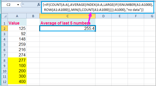
=IF(COUNT(A:A),AVERAGE(INDEX(A:A,LARGE(IF(ISNUMBER(A1:A10000),ROW(A1:A10000)),MIN(5,COUNT(A1:A10000)))):A10000),"no data") (A: A คือคอลัมน์ที่มีข้อมูลที่คุณใช้ A1: A10000 เป็นช่วงไดนามิกคุณสามารถขยายได้ตราบเท่าที่คุณต้องการและจำนวน 5 ระบุค่า n สุดท้าย) จากนั้นกด Ctrl + Shift + Enter คีย์เข้าด้วยกันเพื่อรับค่าเฉลี่ยของตัวเลข 5 ตัวสุดท้าย ดูภาพหน้าจอ:

และตอนนี้เมื่อคุณป้อนตัวเลขใหม่หลังข้อมูลเดิมค่าเฉลี่ยจะเปลี่ยนไปเช่นกันดูภาพหน้าจอ:
หมายเหตุ: ถ้าคอลัมน์ของเซลล์มี 0 ค่าคุณต้องการยกเว้นค่า 0 จากตัวเลข 5 ตัวสุดท้ายของคุณสูตรข้างต้นจะใช้ไม่ได้ที่นี่ฉันสามารถแนะนำสูตรอาร์เรย์อื่นให้คุณเพื่อรับค่าเฉลี่ย 5 ค่าสุดท้ายที่ไม่ใช่ศูนย์ โปรดป้อนสูตรนี้:
=AVERAGE(SUBTOTAL(9,OFFSET(A1:A10000,LARGE(IF(A1:A10000>0,ROW(A1:A10000)-MIN(ROW(A1:A10000))),ROW(INDIRECT("1:5"))),0,1)))จากนั้นกด Ctrl + Shift + Enter คีย์เพื่อให้ได้ผลลัพธ์ที่คุณต้องการดูภาพหน้าจอ:

บทความที่เกี่ยวข้อง:
วิธีการเฉลี่ยทุกๆ 5 แถวหรือคอลัมน์ใน Excel
วิธีการเฉลี่ยค่า 3 อันดับบนหรือล่างใน Excel
สุดยอดเครื่องมือเพิ่มผลผลิตในสำนักงาน
เพิ่มพูนทักษะ Excel ของคุณด้วย Kutools สำหรับ Excel และสัมผัสประสิทธิภาพอย่างที่ไม่เคยมีมาก่อน Kutools สำหรับ Excel เสนอคุณสมบัติขั้นสูงมากกว่า 300 รายการเพื่อเพิ่มประสิทธิภาพและประหยัดเวลา คลิกที่นี่เพื่อรับคุณสมบัติที่คุณต้องการมากที่สุด...
")
แท็บ Office นำอินเทอร์เฟซแบบแท็บมาที่ Office และทำให้งานของคุณง่ายขึ้นมาก
- เปิดใช้งานการแก้ไขและอ่านแบบแท็บใน Word, Excel, PowerPoint, ผู้จัดพิมพ์, Access, Visio และโครงการ
- เปิดและสร้างเอกสารหลายรายการในแท็บใหม่ของหน้าต่างเดียวกันแทนที่จะเป็นในหน้าต่างใหม่
- เพิ่มประสิทธิภาพการทำงานของคุณ 50% และลดการคลิกเมาส์หลายร้อยครั้งให้คุณทุกวัน!
")