ไปยังเนื้อหาหลัก

วิธีการ sumif เซลล์ที่อยู่ติดกันมีค่าเท่ากันว่างเปล่าหรือมีข้อความใน Excel?

ในขณะที่ใช้ Microsoft Excel คุณอาจต้องรวมค่าที่เซลล์ที่อยู่ติดกันเท่ากับเกณฑ์ในช่วงหนึ่งหรือรวมค่าที่เซลล์ที่อยู่ติดกันว่างเปล่าหรือมีข้อความอยู่ ในบทช่วยสอนนี้เราจะให้สูตรเพื่อจัดการกับปัญหาเหล่านี้

เซลล์ที่อยู่ติดกัน Sumif เท่ากับเกณฑ์ใน Excel
เซลล์ที่อยู่ติดกัน Sumif ว่างเปล่าใน Excel
เซลล์ Sumif ที่อยู่ติดกันมีข้อความใน Excel


เซลล์ที่อยู่ติดกัน Sumif เท่ากับเกณฑ์ใน Excel

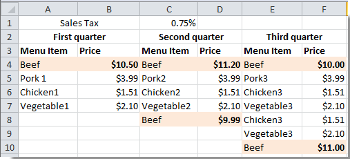
ตามที่แสดงภาพหน้าจอคุณจะต้องรวมราคาทั้งหมดของ Beef กรุณาดำเนินการดังนี้

1. ระบุเซลล์สำหรับแสดงผลลัพธ์

2. คัดลอกและวางสูตร =SUM(IF(A4:E10=A13, B4:F10, 0)) เข้าไปใน สูตรบาร์จากนั้นกด Ctrl + เปลี่ยน + ป้อนคีย์พร้อมกันเพื่อให้ได้ผลลัพธ์

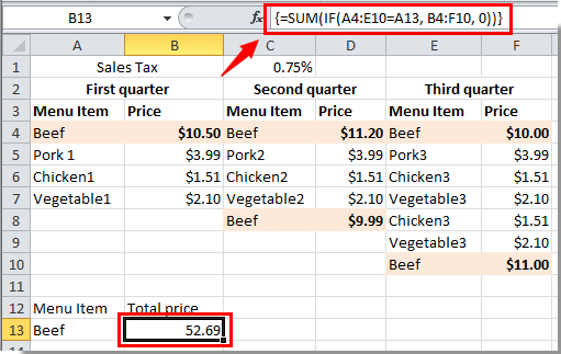
หมายเหตุ: ในสูตร A4: E10 คือช่วงข้อมูลที่มีเกณฑ์เฉพาะที่คุณต้องการ A13 คือเกณฑ์ที่คุณต้องการรวมเซลล์ตามและ B4: F10 คือช่วงที่มีค่าที่คุณต้องการรวม . โปรดเปลี่ยนช่วงตามข้อมูลของคุณเอง


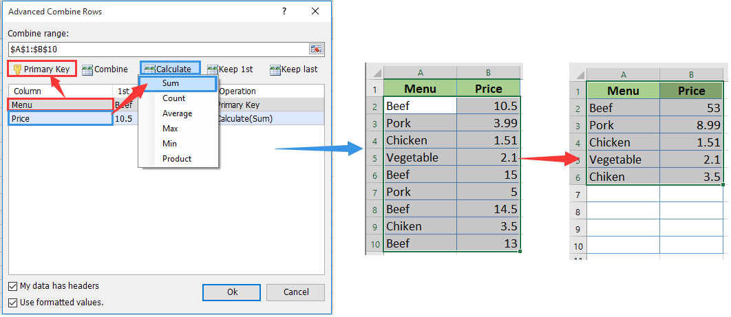
รวมรายการที่ซ้ำกันในคอลัมน์ได้อย่างง่ายดายและรวมค่าในคอลัมน์อื่นตามรายการที่ซ้ำกันใน Excel

พื้นที่ Kutools สำหรับ Excel's แถวรวมขั้นสูง ยูทิลิตี้ช่วยให้คุณสามารถรวมแถวที่ซ้ำกันในคอลัมน์และคำนวณหรือรวมค่าในคอลัมน์อื่นโดยยึดตามรายการที่ซ้ำกันใน Excel
ดาวน์โหลดและทดลองใช้ทันที! (เส้นทางฟรี 30 วัน)


เซลล์ที่อยู่ติดกัน Sumif ว่างเปล่าใน Excel

ตัวอย่างเช่นคุณมีช่วง A2: B7 และคุณเพียงแค่ต้องรวมค่าที่เซลล์ที่อยู่ติดกันว่าง ดูภาพหน้าจอด้านล่าง คุณต้องดำเนินการดังนี้

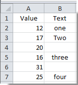
1. เลือกเซลล์ว่างเพื่อแสดงผลลัพธ์ คัดลอกและวางสูตร = SUM (IF (ISBLANK (B2: B7), A2: A7,0)) (B2: B7 คือช่วงข้อมูลที่มีเซลล์ว่างและ A2: A7 คือข้อมูลที่คุณต้องการรวม) ในแถบสูตรจากนั้นกด Ctrl + เปลี่ยน + เข้าสู่ คีย์ในเวลาเดียวกันเพื่อให้ได้ผลลัพธ์

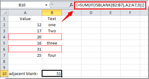
จากนั้นคุณจะเห็นค่าทั้งหมดที่เซลล์ที่อยู่ติดกันว่างจะถูกรวมและแสดงในเซลล์ที่ระบุ

เซลล์ Sumif ที่อยู่ติดกันมีข้อความใน Excel

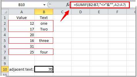
วิธีการข้างต้นช่วยให้คุณรวมค่าที่เซลล์ที่อยู่ติดกันว่างเปล่าในช่วงหนึ่ง ในส่วนนี้คุณจะได้เรียนรู้วิธีการรวมค่าที่เซลล์ที่อยู่ติดกันมีข้อความใน Excel

เพียงใช้ตัวอย่างเดียวกับวิธีการด้านบนที่แสดง

1. เลือกเซลล์ว่างคัดลอกและวางสูตร = SUMIF (B2: B7, "<>" & "", A2: A7) (B2: B7 คือช่วงข้อมูลที่มีเซลล์ข้อความและ A2: A7 คือข้อมูลที่คุณต้องการรวม) ในแถบสูตรจากนั้นกด Ctrl + เปลี่ยน + เข้าสู่ กุญแจ

คุณจะเห็นค่าทั้งหมดที่เซลล์ที่อยู่ติดกันมีข้อความถูกสรุปและแสดงในเซลล์ที่เลือก

สุดยอดเครื่องมือเพิ่มผลผลิตในสำนักงาน

🤖 Kutools AI ผู้ช่วย: ปฏิวัติการวิเคราะห์ข้อมูลโดยยึดตาม: การดำเนินการที่ชาญฉลาด   |  สร้างรหัส  |  สร้างสูตรที่กำหนดเอง  |  วิเคราะห์ข้อมูลและสร้างแผนภูมิ  |  เรียกใช้ฟังก์ชัน Kutools...
คุณสมบัติยอดนิยม: ค้นหา เน้น หรือระบุรายการที่ซ้ำกัน   |  ลบแถวว่าง   |  รวมคอลัมน์หรือเซลล์โดยไม่สูญเสียข้อมูล   |   รอบโดยไม่มีสูตร ...
การค้นหาขั้นสูง: VLookup หลายเกณฑ์    VLookup หลายค่า  |   VLookup ข้ามหลายแผ่น   |   การค้นหาที่ไม่ชัดเจน ....
รายการแบบเลื่อนลงขั้นสูง: สร้างรายการแบบหล่นลงอย่างรวดเร็ว   |  รายการแบบหล่นลงขึ้นอยู่กับ   |  เลือกหลายรายการแบบหล่นลง ....
ผู้จัดการคอลัมน์: เพิ่มจำนวนคอลัมน์เฉพาะ  |  ย้ายคอลัมน์  |  สลับสถานะการมองเห็นของคอลัมน์ที่ซ่อนอยู่  |  เปรียบเทียบช่วงและคอลัมน์ ...
คุณสมบัติเด่น: กริดโฟกัส   |  มุมมองการออกแบบ   |   บาร์สูตรใหญ่    สมุดงานและตัวจัดการชีต   |  ห้องสมุดทรัพยากร (ข้อความอัตโนมัติ)   |  เลือกวันที่   |  รวมแผ่นงาน   |  เข้ารหัส/ถอดรหัสเซลล์    ส่งอีเมลตามรายการ   |  ซุปเปอร์ฟิลเตอร์   |   ตัวกรองพิเศษ (กรองตัวหนา/ตัวเอียง/ขีดทับ...) ...
ชุดเครื่องมือ 15 อันดับแรก12 ข้อความ เครื่องมือ (เพิ่มข้อความ, ลบอักขระ, ... )   |   50 + แผนภูมิ ประเภท (แผนภูมิ Gantt, ... )   |   40+ ใช้งานได้จริง สูตร (คำนวณอายุตามวันเกิด, ... )   |   19 การแทรก เครื่องมือ (ใส่ QR Code, แทรกรูปภาพจากเส้นทาง, ... )   |   12 การแปลง เครื่องมือ (ตัวเลขเป็นคำ, การแปลงสกุลเงิน, ... )   |   7 ผสานและแยก เครื่องมือ (แถวรวมขั้นสูง, แยกเซลล์, ... )   |   ... และอื่น ๆ

เพิ่มพูนทักษะ Excel ของคุณด้วย Kutools สำหรับ Excel และสัมผัสประสิทธิภาพอย่างที่ไม่เคยมีมาก่อน Kutools สำหรับ Excel เสนอคุณสมบัติขั้นสูงมากกว่า 300 รายการเพื่อเพิ่มประสิทธิภาพและประหยัดเวลา  คลิกที่นี่เพื่อรับคุณสมบัติที่คุณต้องการมากที่สุด...

รายละเอียด


แท็บ Office นำอินเทอร์เฟซแบบแท็บมาที่ Office และทำให้งานของคุณง่ายขึ้นมาก

  • เปิดใช้งานการแก้ไขและอ่านแบบแท็บใน Word, Excel, PowerPoint, ผู้จัดพิมพ์, Access, Visio และโครงการ
  • เปิดและสร้างเอกสารหลายรายการในแท็บใหม่ของหน้าต่างเดียวกันแทนที่จะเป็นในหน้าต่างใหม่
  • เพิ่มประสิทธิภาพการทำงานของคุณ 50% และลดการคลิกเมาส์หลายร้อยครั้งให้คุณทุกวัน!
Comments (14)
No ratings yet. Be the first to rate!
This comment was minimized by the moderator on the site
Sumif Adjacent Cell Equals A Criterion In Excel formula is not working for me, it is adding everything instead of just the cells with data we want.
This comment was minimized by the moderator on the site
Hi Cole,
Which Excel version are you using? Would you mind providing a screenshot of your data?
This comment was minimized by the moderator on the site
Hello I am trying to set up a pricing list. I have used a dropdown list for the selected products. How do I make excel input a price based on the choice of the text in the dropdown list.
This comment was minimized by the moderator on the site
Hi erin,
Methods in this article can help you. Please have a try: https://www.extendoffice.com/documents/excel/2400-excel-drop-down-list-auto-populate.html
This comment was minimized by the moderator on the site
I am trying to get a return value of "yes" if A1:A7 contains any text. What formulas can I use?
This comment was minimized by the moderator on the site
Dear Wyman Thomas,
Supposing you need to return value of "Yes" if cell A1 contains "Apple", this formula can help you =IF(ISNUMBER(SEARCH("Apple",A1)), "Yes", "No").
This comment was minimized by the moderator on the site
Pretty sure

=SUMIF(B2:B7,"<>"&"",A2:B7) should be


=SUMIF(B2:B7,"<>"&"",A2:A7)
This comment was minimized by the moderator on the site
Few People Notice that, We take it A2:A7
This comment was minimized by the moderator on the site
Hi,
Thank you for your reminding.
This comment was minimized by the moderator on the site
Dear all. I would like to use the SUMIF function in the following way: -Sum range is 1:1 -Criteria Range is 2:2 -Criteria is "jorge" However, I would like the function o work a little bit different. If "jorge" is found on B2, I would like A1 to be sum instead of A2. I tried =SUMIF(1:1,OFFSET(2:2,,1),"jorge") but excel does not accept such criteria range argument. How to get it working?
This comment was minimized by the moderator on the site
I am looking to create a budget spreadsheet. My goal is to plug in my daily expenses, with the category in one cell and the amount in the cell beneath. As far as my spending goes, I have no problem calculating. However, I am struggling with a formula to create a running tally of each category. Can you help?
This comment was minimized by the moderator on the site
Mike I am working on the same problem I created a drop down list for column D and my costs are in column C. Simply change the name (Contracts) of the formula to your category name. =SUMIF(D2:D31,""Contracts"",C2:C31)
This comment was minimized by the moderator on the site
hi, hope you could help me on this i want to create a formula where-in the codes under the subnet, be reflected on the net. see below place(net) 1 place1 2 place2 3 place3 4 place4 5 place5 where place net should have a code 1+2+3+4+5, i know how to concatenate and use "&" but i need to have a formula where i could drag it down since its not the only net in my specs, hoping for your answer? bog thanks regards, jayson
This comment was minimized by the moderator on the site
I would like to get the return value "yes" if the cells in A1:A7 contain data. What formula can I use?
There are no comments posted here yet
Please leave your comments in English
Posting as Guest
×
Rate this post:
0   Characters
Suggested Locations