ไปยังเนื้อหาหลัก

วิธีสร้างหมายเลขสุ่มโดยไม่ซ้ำกันใน Excel

ในหลาย ๆ กรณีคุณอาจต้องการสร้างตัวเลขสุ่มใน Excel? แต่ด้วยสูตรทั่วไปในการสุ่มตัวเลขอาจมีบางค่าที่ซ้ำกัน ที่นี่ฉันจะบอกคุณเทคนิคบางอย่างในการสร้างตัวเลขสุ่มโดยไม่ซ้ำกันใน Excel

สร้างตัวเลขสุ่มที่ไม่ซ้ำกันด้วยสูตร

สร้างหมายเลขสุ่มที่ไม่ซ้ำใครด้วย Kutools สำหรับ Excel's Insert Random Data (Easy!) ความคิดที่ดี 3


ลูกศรสีฟ้าฟองขวา สร้างตัวเลขสุ่มที่ไม่ซ้ำกันด้วยสูตร

ในการสร้างตัวเลขสุ่มที่ไม่ซ้ำกันใน Excel คุณต้องใช้สองสูตร

1. สมมติว่าคุณต้องการสร้างตัวเลขสุ่มโดยไม่ซ้ำกันในคอลัมน์ A และคอลัมน์ B ตอนนี้เลือกเซลล์ E1 แล้วพิมพ์สูตรนี้ = RAND ()จากนั้นกด เข้าสู่ สำคัญดูภาพหน้าจอ:
doc-สุ่ม-ไม่-ซ้ำ-1

2. และเลือกทั้งคอลัมน์ E โดยการกด Ctrl + ช่องว่าง พร้อมกันจากนั้นกด Ctrl + D คีย์เพื่อใช้สูตร = RAND () ทั้งคอลัมน์ E. ดูภาพหน้าจอ:
doc-สุ่ม-ไม่-ซ้ำ-2

3. จากนั้นในเซลล์ D1 พิมพ์จำนวนสุ่มสูงสุดที่คุณต้องการ ในกรณีนี้ฉันต้องการแทรกตัวเลขสุ่มโดยไม่ต้องซ้ำระหว่าง 1 ถึง 50 ดังนั้นฉันจะพิมพ์ 50 ลงใน D1
doc-สุ่ม-ไม่-ซ้ำ-3

4. ไปที่คอลัมน์ A เลือกเซลล์ A1 พิมพ์สูตรนี้ =IF(ROW()-ROW(A$1)+1>$D$1/2,"",RANK(OFFSET($E$1,ROW()-ROW(A$1)+(COLUMN()-COLUMN($A1))*($D$1/2),),$E$1:INDEX($E$1:$E$1000,$D$1)))จากนั้นลากจุดจับเติมไปยังคอลัมน์ B ถัดไปแล้วลากที่จับเติมลงไปในช่วงที่คุณต้องการ ดูภาพหน้าจอ:
doc-สุ่ม-ไม่-ซ้ำ-4

ตอนนี้ในช่วงนี้ตัวเลขสุ่มที่คุณต้องการจะไม่ซ้ำ

หมายเหตุ

1. ในสูตรยาวด้านบน A1 ระบุเซลล์ที่คุณใช้สูตรยาว D1 ระบุจำนวนสูงสุดของตัวเลขสุ่ม E1 คือเซลล์แรกของคอลัมน์ที่คุณใช้สูตร = RAND () และ 2 ระบุว่าคุณต้องการแทรก สุ่มตัวเลขเป็นสองคอลัมน์ คุณสามารถเปลี่ยนได้ตามความต้องการของคุณ

2. เมื่อตัวเลขที่ไม่ซ้ำกันทั้งหมดถูกสร้างขึ้นในช่วงเซลล์ที่ซ้ำซ้อนจะแสดงเป็นช่องว่าง

3. ด้วยวิธีนี้คุณสามารถสร้างหมายเลขสุ่มเริ่มต้นจากหมายเลข 1 แต่ด้วยวิธีที่สองคุณสามารถระบุช่วงตัวเลขสุ่มได้อย่างง่ายดาย


ลูกศรสีฟ้าฟองขวา สร้างหมายเลขสุ่มที่ไม่ซ้ำกันด้วย Kutools สำหรับ Excel's Insert Random Data

ด้วยสูตรข้างต้นมีความไม่สะดวกในการจัดการมากเกินไป แต่ด้วย Kutools สำหรับ Excel's แทรกข้อมูลสุ่ม คุณสามารถแทรกตัวเลขสุ่มที่ไม่ซ้ำกันได้อย่างรวดเร็วและง่ายดายตามที่คุณต้องการซึ่งจะช่วยประหยัดเวลาได้มาก

ใช้เวลาน้อยลง แต่ให้ผลผลิตสูงขึ้น

รวมเครื่องมือระดับมืออาชีพมากกว่า 300 รายการสำหรับ Excel 2019-2003
1.0 เวอร์ชันแรกเปิดตัวในปี 2011 ตอนนี้เป็นเวอร์ชัน 18.0
แก้งานที่ซับซ้อนประจำวันของ Excel ส่วนใหญ่ในไม่กี่วินาทีประหยัดเวลาของคุณ
ทดลองใช้ฟรี 30 วันโดยไม่มีข้อ จำกัด ใด ๆ

kte 包装盒

หลังจากการติดตั้ง Kutools สำหรับ Excel โปรดทำดังนี้:(ดาวน์โหลด Kutools for Excel ฟรีทันที!)

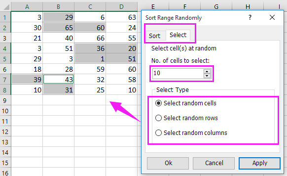
1. เลือกช่วงที่คุณต้องการสร้างตัวเลขสุ่มแล้วคลิก Kutools > สิ่งที่ใส่เข้าไป > แทรกข้อมูลสุ่ม. ดูภาพหน้าจอ:

2 ใน แทรกข้อมูลสุ่ม ใหไปที่ จำนวนเต็ม พิมพ์ช่วงตัวเลขที่คุณต้องการลงในไฟล์ จาก และ ไปยัง กล่องข้อความและอย่าลืมตรวจสอบ ค่าที่ไม่ซ้ำกัน ตัวเลือก ดูภาพหน้าจอ:

3 คลิก Ok เพื่อสร้างตัวเลขสุ่มและออกจากกล่องโต้ตอบ

หมายเหตุถ้าเซลล์ที่คุณเลือกมากกว่าตัวเลขสุ่มเซลล์ที่ซ้ำซ้อนจะแสดงเป็นว่างเปล่า

คุณยังสามารถแทรกวันที่ที่ไม่ซ้ำแบบสุ่มเวลาที่ไม่ซ้ำแบบสุ่มโดย แทรกข้อมูลสุ่ม. หากคุณต้องการทดลองใช้ฟรี แทรกข้อมูลสุ่ม, โปรดดาวน์โหลดเดี๋ยวนี้!
แทรกข้อมูลแบบสุ่ม

เคล็ดลับหากคุณต้องการเลือกหรือจัดเรียงข้อมูลแบบสุ่มโปรดลองใช้ Kutools for Excel's จัดเรียงช่วงแบบสุ่ม ดังที่แสดงในภาพหน้าจอต่อไปนี้ ฟังก์ชั่นเต็มรูปแบบโดยไม่มีข้อ จำกัด ใน 30 วัน โปรดดาวน์โหลดและทดลองใช้ฟรีทันที

doc เลือกแบบสุ่ม


ลูกศรสีฟ้าฟองขวา แทรกข้อมูลแบบสุ่มโดยไม่ต้องทำซ้ำ


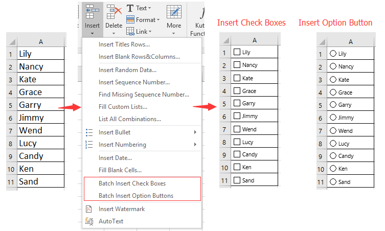
แทรกช่องทำเครื่องหมายหรือปุ่มต่างๆลงในช่วงของเซลล์ในแผ่นงานได้อย่างรวดเร็ว

ใน Excel คุณสามารถแทรกช่องทำเครื่องหมาย / ปุ่มลงในเซลล์ได้เพียงครั้งเดียวซึ่งจะเป็นปัญหาหากมีหลายเซลล์ที่ต้องแทรกช่องทำเครื่องหมาย / ปุ่มในเวลาเดียวกัน Kutools สำหรับ Excel มียูทิลิตี้ที่มีประสิทธิภาพ - ตรวจสอบการแทรกแบทช์ กล่อง / ปุ่มตัวเลือกแทรกแบทช์ สามารถแทรกช่องทำเครื่องหมาย / ปุ่มลงในเซลล์ที่เลือกได้ด้วยคลิกเดียว  คลิกเพื่อทดลองใช้ฟีเจอร์เต็มรูปแบบฟรีใน 30 วัน!
doc แทรกปุ่มตัวเลือกกล่องกาเครื่องหมาย
 
Kutools for Excel: มีโปรแกรมเสริม Excel ที่มีประโยชน์มากกว่า 300 รายการให้ทดลองใช้ฟรีโดยไม่มีข้อ จำกัด ใน 30 วัน

สุดยอดเครื่องมือเพิ่มผลผลิตในสำนักงาน

🤖 Kutools AI ผู้ช่วย: ปฏิวัติการวิเคราะห์ข้อมูลโดยยึดตาม: การดำเนินการที่ชาญฉลาด   |  สร้างรหัส  |  สร้างสูตรที่กำหนดเอง  |  วิเคราะห์ข้อมูลและสร้างแผนภูมิ  |  เรียกใช้ฟังก์ชัน Kutools...
คุณสมบัติยอดนิยม: ค้นหา เน้น หรือระบุรายการที่ซ้ำกัน   |  ลบแถวว่าง   |  รวมคอลัมน์หรือเซลล์โดยไม่สูญเสียข้อมูล   |   รอบโดยไม่มีสูตร ...
การค้นหาขั้นสูง: VLookup หลายเกณฑ์    VLookup หลายค่า  |   VLookup ข้ามหลายแผ่น   |   การค้นหาที่ไม่ชัดเจน ....
รายการแบบเลื่อนลงขั้นสูง: สร้างรายการแบบหล่นลงอย่างรวดเร็ว   |  รายการแบบหล่นลงขึ้นอยู่กับ   |  เลือกหลายรายการแบบหล่นลง ....
ผู้จัดการคอลัมน์: เพิ่มจำนวนคอลัมน์เฉพาะ  |  ย้ายคอลัมน์  |  สลับสถานะการมองเห็นของคอลัมน์ที่ซ่อนอยู่  |  เปรียบเทียบช่วงและคอลัมน์ ...
คุณสมบัติเด่น: กริดโฟกัส   |  มุมมองการออกแบบ   |   บาร์สูตรใหญ่    สมุดงานและตัวจัดการชีต   |  ห้องสมุดทรัพยากร (ข้อความอัตโนมัติ)   |  เลือกวันที่   |  รวมแผ่นงาน   |  เข้ารหัส/ถอดรหัสเซลล์    ส่งอีเมลตามรายการ   |  ซุปเปอร์ฟิลเตอร์   |   ตัวกรองพิเศษ (กรองตัวหนา/ตัวเอียง/ขีดทับ...) ...
ชุดเครื่องมือ 15 อันดับแรก12 ข้อความ เครื่องมือ (เพิ่มข้อความ, ลบอักขระ, ... )   |   50 + แผนภูมิ ประเภท (แผนภูมิ Gantt, ... )   |   40+ ใช้งานได้จริง สูตร (คำนวณอายุตามวันเกิด, ... )   |   19 การแทรก เครื่องมือ (ใส่ QR Code, แทรกรูปภาพจากเส้นทาง, ... )   |   12 การแปลง เครื่องมือ (ตัวเลขเป็นคำ, การแปลงสกุลเงิน, ... )   |   7 ผสานและแยก เครื่องมือ (แถวรวมขั้นสูง, แยกเซลล์, ... )   |   ... และอื่น ๆ

เพิ่มพูนทักษะ Excel ของคุณด้วย Kutools สำหรับ Excel และสัมผัสประสิทธิภาพอย่างที่ไม่เคยมีมาก่อน Kutools สำหรับ Excel เสนอคุณสมบัติขั้นสูงมากกว่า 300 รายการเพื่อเพิ่มประสิทธิภาพและประหยัดเวลา  คลิกที่นี่เพื่อรับคุณสมบัติที่คุณต้องการมากที่สุด...

รายละเอียด


แท็บ Office นำอินเทอร์เฟซแบบแท็บมาที่ Office และทำให้งานของคุณง่ายขึ้นมาก

  • เปิดใช้งานการแก้ไขและอ่านแบบแท็บใน Word, Excel, PowerPoint, ผู้จัดพิมพ์, Access, Visio และโครงการ
  • เปิดและสร้างเอกสารหลายรายการในแท็บใหม่ของหน้าต่างเดียวกันแทนที่จะเป็นในหน้าต่างใหม่
  • เพิ่มประสิทธิภาพการทำงานของคุณ 50% และลดการคลิกเมาส์หลายร้อยครั้งให้คุณทุกวัน!
Comments (17)
No ratings yet. Be the first to rate!
This comment was minimized by the moderator on the site
En la parte Genere números aleatorios únicos con fórmulas como hago para ampliar el numero de columnas pasar de 2 a 5 sin repetir los numeros segun la formula que ud puso: =IF(ROW()-ROW(A$1)+1>$D$1/2,"",RANK(OFFSET($E$1,ROW()-ROW(A$1)+(COLUMN()-COLUMN($A1))*($D$1/2),),$E$1:INDEX($E$1:$E$1000,$D$1)))
This comment was minimized by the moderator on the site
Hello. I just found this site, and am trying to figure out best way to assign a new code to people. I'd like to assign a random code for people to use between 1000 and 65000, that does not equal any codes already assigned. I'd also like it to be formatted with 5 numbers (00000), but that's not a big deal if it doesn't take care of that. Any ideas on how to make this work? TIA :-)
This comment was minimized by the moderator on the site
Hi, Janel, why you donot try the Data Validation in Excel? It can only allow whole numbers between 1000 and 65000 to be entered in a cell range.
This comment was minimized by the moderator on the site
Help anyone :-) This one I cannot figure out. At our school we often put together students in groups - 2 and 2 together for a number of working sessions. 9 in this case. There are 18 students (vary) in the class. What I am chasing is a formula that gives me a random result of who should work together in the 9 working sessions without having students meeting each other twice. So I need Excel to give me a result of 18 students spread across 9 working sessions and any student must not be match with another student twice. How the xxxx do I fix that? I have search all over the place for inspiration without luck. Any input is appreciated :-)
This comment was minimized by the moderator on the site
Hi, Anders, you need to list all names in column A, then in column B, apply formula =rand(), then specify 2 as the size in cell F2, now apply this formula =ROUNDUP(RANK(B3,$B$3:$B$19)/$F$2,0) in column C as below screenshot shown
This comment was minimized by the moderator on the site
Hi. Thanks for your reply.
I understand you suggestions, but how do I achieve a setup where all students are assigned to maksimum number of workshops where 2 students are randomly assigned to first one workshop, then the second workshop, then the third workshop etc. etc. and to take this even further a student must not be matched with another student that he/she already have worked with. So when having 18 students I need "the system" to allocate all student to (in this case) 9 workshop (e.g. one workshop per week) and no student should be a student they have already worked with.
This comment was minimized by the moderator on the site
Hi there, did you ever manage to work out a solution to this, I've encountered the same issue. Any help would be appreciated.
This comment was minimized by the moderator on the site
Or you could use a sudoku setup.
This comment was minimized by the moderator on the site
How can I do the same thing with a custom list? Not numbers?
This comment was minimized by the moderator on the site
Your custom list is in Column A. Lets say it has 100 values and it is located in A1:A100

Column B is a counter:
1 for B1 and (B1+1) for B2:B100

Column C is a random list:
RAND() for C1:C100

Column D is a random rank based on the random list:
RANK.EQ(C1;$C$1:$C$100)

Column E is your output:
INDEX($A$1:$A$100;MATCH(D1;$B$1:$B$100;0))

Note: There is virtually no chance of generating a duplicate value on column C since RAND() have billions of possibilities. But, if you really want to erase that chance you can type the following formula at column D2:D100
IF(COUNTIFS($C$2:C2;C2)>0;D1+1;RANK.EQ(C2;$C$1:$C$100))
This comment was minimized by the moderator on the site
I need to create 5000 random numbers 1-90 no duplicates 30 columes I and using the formula =RAND() and =IF(ROW()-ROW(A$1)+1>$D$1/2,"",RANK(OFFSET($E$1,ROW()-ROW(A$1)+(COLUMN()-COLUMN($A1))*($D$1/2),),$E$1:INDEX($E$1:$E$1000,$D$1))) is there way that i could change the formula to extract the 5000 numbers
This comment was minimized by the moderator on the site
Sorry I have no idea, you can place this problem to our forum https://www.extendoffice.com/forum.html, maybe someone can help you.
This comment was minimized by the moderator on the site
After about three hours of trying to completely understand the long complicated formula to generate random numbers without duplicates, I figured out a far simpler formula that has the same results. After you randomly generate the numbers in a column using the RAND() function, You can simplify the formula:=IF(ROW()-ROW(A$1)+1>$D$1/2,"",RANK(OFFSET($E$1,ROW()-ROW(A$1)+(COLUMN()-COLUMN($A1))*($D$1/2),),$E$1:INDEX($E$1:$E$1000,$D$1))) in cell a1 to =Rank(E1,$E$1:$E$50). Then if you would like 50 random generated "unique numbers." you simply drag the formula through column a to cell a50. It is a lot simpler. Thank you for answering my question regardless of the huge unneeded formula. If you did not have this website. I don't think I would have been able to solve my problem. #WAR Jiggly
This comment was minimized by the moderator on the site
Actually, if you have two equal values, rank will give the same value to both. Rank formula does return repeated rank values.
This comment was minimized by the moderator on the site
Manuel Ramirez.

The formula RAND() has hundreds of billions of possibilities, but even so you can use a conditional to not repeat the numbers:
A1 = Rank(E1,$E$1:$E$50)
A2 = IF(COUNTIFS($E$1:E1;E1)>1;A1+1;Rank(E2,$E$1:$E$50)
This comment was minimized by the moderator on the site
Hi, Base on Generate unique random numbers with formulas , How can I specify the starting point of a random number? Let's say I want to random "15 to 30".
This comment was minimized by the moderator on the site
Use RANDBETWEEN() to get random numbers lies between two numbers.
There are no comments posted here yet
Please leave your comments in English
Posting as Guest
×
Rate this post:
0   Characters
Suggested Locations