วิธีการรวมค่าตามเกณฑ์ข้อความใน Excel
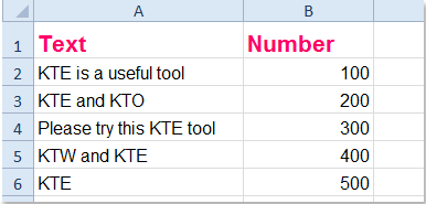
ใน Excel คุณเคยพยายามรวมค่าตามคอลัมน์อื่นของเกณฑ์ข้อความหรือไม่? ตัวอย่างเช่นฉันมีช่วงของข้อมูลในแผ่นงานดังภาพหน้าจอต่อไปนี้ที่แสดงตอนนี้ฉันต้องการเพิ่มตัวเลขทั้งหมดในคอลัมน์ B ที่สอดคล้องกับค่าข้อความในคอลัมน์ A ที่ตรงตามเกณฑ์ที่กำหนดเช่นรวมตัวเลขหาก เซลล์ในคอลัมน์ A มี KTE
 |
รวมค่าตามคอลัมน์อื่นหากมีข้อความบางข้อความ รวมค่าตามคอลัมน์อื่นหากขึ้นต้นด้วยข้อความบางข้อความ |
 รวมค่าตามคอลัมน์อื่นหากมีข้อความบางข้อความ
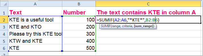
ลองใช้ข้อมูลข้างต้นเพื่อเพิ่มค่าทั้งหมดเข้าด้วยกันซึ่งมีข้อความ“ KTE” ในคอลัมน์ A สูตรต่อไปนี้อาจช่วยคุณได้:
กรุณาใส่สูตรนี้ = SUMIF (A2: A6, "* KTE *", B2: B6) ลงในเซลล์ว่างแล้วกด เข้าสู่ จากนั้นตัวเลขทั้งหมดในคอลัมน์ B ที่เซลล์ที่เกี่ยวข้องในคอลัมน์ A มีข้อความ "KTE" จะรวมกัน ดูภาพหน้าจอ:
 |
 |
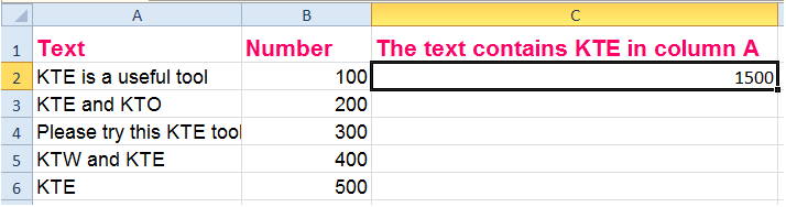 |
ปลาย: ในสูตรข้างต้น A2: A6 คือช่วงข้อมูลที่คุณเพิ่มค่าตาม * KTE * หมายถึงเกณฑ์ที่คุณต้องการและ B2: B6 คือช่วงที่คุณต้องการรวม
รวมค่าตามคอลัมน์อื่นหากขึ้นต้นด้วยข้อความบางข้อความ
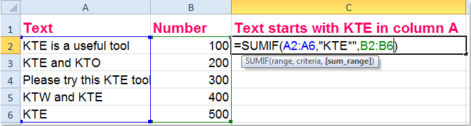
หากคุณต้องการรวมค่าเซลล์ในคอลัมน์ B โดยที่เซลล์ที่เกี่ยวข้องในคอลัมน์ A ซึ่งข้อความขึ้นต้นด้วย "KTE" คุณสามารถใช้สูตรนี้ได้: = SUMIF (A2: A6, "KTE *", B2: B6)ดูภาพหน้าจอ:
 |
|
 |
ปลาย: ในสูตรข้างต้น A2: A6 คือช่วงข้อมูลที่คุณเพิ่มค่าตาม KTE * หมายถึงเกณฑ์ที่คุณต้องการและ B2: B6 คือช่วงที่คุณต้องการรวม
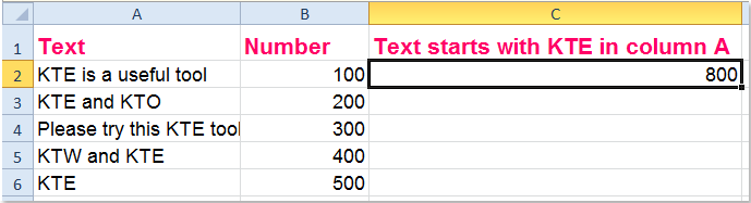
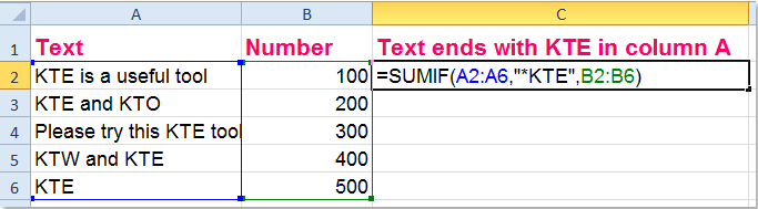
รวมค่าตามคอลัมน์อื่นหากลงท้ายด้วยข้อความบางข้อความ
หากต้องการเพิ่มค่าทั้งหมดในคอลัมน์ B โดยที่เซลล์ที่เกี่ยวข้องในคอลัมน์ A ซึ่งข้อความลงท้ายด้วย "KTE" สูตรนี้สามารถช่วยคุณได้: = SUMIF (A2: A6, "* KTE", B2: B6), (A2: A6 คือช่วงข้อมูลที่คุณเพิ่มค่าตาม KTE * หมายถึงเกณฑ์ที่คุณต้องการและ B2: B6 คือช่วงที่คุณต้องการรวม) ดูภาพหน้าจอ:
 |
|
 |
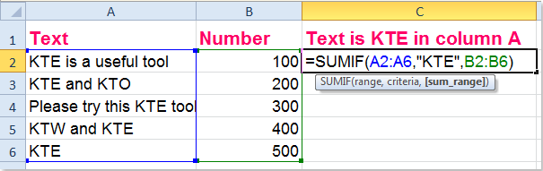
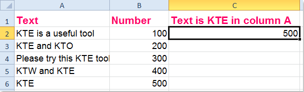
รวมค่าตามคอลัมน์อื่นหากเป็นข้อความบางข้อความ
หากคุณเพียงต้องการรวมค่าในคอลัมน์ B ซึ่งเนื้อหาของเซลล์ที่เกี่ยวข้องเท่านั้นคือ "KTE" ของคอลัมน์ A โปรดใช้สูตรนี้: = SUMIF (A2: A6, "KTE", B2: B6), (A2: A6 คือช่วงข้อมูลที่คุณเพิ่มค่าตาม KTE หมายถึงเกณฑ์ที่คุณต้องการและ B2: B6 คือช่วงที่คุณต้องการรวม) จากนั้นเฉพาะข้อความคือ "KTE" ในคอลัมน์ A ซึ่งจะเพิ่มจำนวนสัมพัทธ์ในคอลัมน์ B ดูภาพหน้าจอ:
 |
|
 |
|
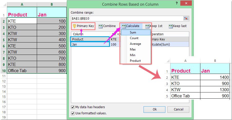
Advanced Combine Rows: (รวมแถวที่ซ้ำกันและผลรวม / ค่าเฉลี่ยที่สอดคล้องกัน):
Kutools สำหรับ Excel: ด้วย Add-in ของ Excel ที่มีประโยชน์มากกว่า 200 รายการให้ทดลองใช้ฟรีโดยไม่มีข้อ จำกัด ใน 60 วัน ดาวน์โหลดและทดลองใช้ฟรีทันที! |
บทความที่เกี่ยวข้อง:
จะรวมทุก n แถวลงใน Excel ได้อย่างไร
วิธีการรวมเซลล์ด้วยข้อความและตัวเลขใน Excel
สุดยอดเครื่องมือเพิ่มผลผลิตในสำนักงาน
เพิ่มพูนทักษะ Excel ของคุณด้วย Kutools สำหรับ Excel และสัมผัสประสิทธิภาพอย่างที่ไม่เคยมีมาก่อน Kutools สำหรับ Excel เสนอคุณสมบัติขั้นสูงมากกว่า 300 รายการเพื่อเพิ่มประสิทธิภาพและประหยัดเวลา คลิกที่นี่เพื่อรับคุณสมบัติที่คุณต้องการมากที่สุด...
")
แท็บ Office นำอินเทอร์เฟซแบบแท็บมาที่ Office และทำให้งานของคุณง่ายขึ้นมาก
- เปิดใช้งานการแก้ไขและอ่านแบบแท็บใน Word, Excel, PowerPoint, ผู้จัดพิมพ์, Access, Visio และโครงการ
- เปิดและสร้างเอกสารหลายรายการในแท็บใหม่ของหน้าต่างเดียวกันแทนที่จะเป็นในหน้าต่างใหม่
- เพิ่มประสิทธิภาพการทำงานของคุณ 50% และลดการคลิกเมาส์หลายร้อยครั้งให้คุณทุกวัน!
")