ไปยังเนื้อหาหลัก

วิธีอัปเดตแผนภูมิอัตโนมัติหลังจากป้อนข้อมูลใหม่ใน Excel

ผู้เขียน: Xiaoyang แก้ไขล่าสุด: 2020-04-26

สมมติว่าคุณได้สร้างแผนภูมิเพื่อติดตามยอดขายประจำวันโดยพิจารณาจากช่วงข้อมูลในสมุดงานของคุณ แต่คุณต้องเปลี่ยนหรือแก้ไขจำนวนข้อมูลทุกวันในกรณีนี้คุณต้องอัปเดตแผนภูมิด้วยตนเองเพื่อให้มีข้อมูลใหม่ มีเคล็ดลับง่ายๆที่จะช่วยให้คุณอัปเดตแผนภูมิโดยอัตโนมัติเมื่อคุณเพิ่มข้อมูลใหม่ลงในช่วงแผนภูมิที่มีอยู่ใน Excel หรือไม่?

อัปเดตแผนภูมิอัตโนมัติหลังจากป้อนข้อมูลใหม่ด้วยการสร้างตาราง

อัปเดตแผนภูมิอัตโนมัติหลังจากป้อนข้อมูลใหม่ด้วยสูตรไดนามิก


ลูกศรสีฟ้าฟองขวา อัปเดตแผนภูมิอัตโนมัติหลังจากป้อนข้อมูลใหม่ด้วยการสร้างตาราง

หากคุณมีช่วงข้อมูลและแผนภูมิคอลัมน์ต่อไปนี้ตอนนี้คุณต้องการให้แผนภูมิอัปเดตโดยอัตโนมัติเมื่อคุณป้อนข้อมูลใหม่ ใน Excel 2007, 2010 หรือ 2013 คุณสามารถสร้างตารางเพื่อขยายช่วงข้อมูลและแผนภูมิจะอัปเดตโดยอัตโนมัติ กรุณาทำตามนี้:

เอกสารอัปเดตแผนภูมิ1

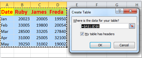
1. เลือกช่วงข้อมูลแล้วคลิก ตาราง ภายใต้ สิ่งที่ใส่เข้าไป ดูภาพหน้าจอ:

เอกสารอัปเดตแผนภูมิ2

2. ใน สร้างตาราง กล่องโต้ตอบหากข้อมูลของคุณมีส่วนหัวโปรดตรวจสอบ ตารางของฉันมีส่วนหัว จากนั้นคลิก OK. ดูภาพหน้าจอ:

เอกสารอัปเดตแผนภูมิ3

3. และช่วงข้อมูลถูกจัดรูปแบบเป็นตารางดูภาพหน้าจอ:

เอกสารอัปเดตแผนภูมิ4

4. ตอนนี้เมื่อคุณเพิ่มค่าสำหรับเดือนมิถุนายนและแผนภูมิจะอัปเดตโดยอัตโนมัติ ดูภาพหน้าจอ:

เอกสารอัปเดตแผนภูมิ5

หมายเหตุ:

1. ข้อมูลที่ป้อนใหม่ของคุณต้องอยู่ติดกับข้อมูลด้านบนหมายความว่าไม่มีแถวหรือคอลัมน์ว่างระหว่างข้อมูลใหม่และข้อมูลที่มีอยู่

2. ในตารางคุณสามารถแทรกข้อมูลระหว่างค่าที่มีอยู่ได้


ลูกศรสีฟ้าฟองขวา อัปเดตแผนภูมิอัตโนมัติหลังจากป้อนข้อมูลใหม่ด้วยสูตรไดนามิก

แต่บางครั้งคุณไม่ต้องการเปลี่ยนช่วงเป็นตารางและวิธีการข้างต้นไม่สามารถใช้ได้ใน Excel 2003 หรือเวอร์ชันก่อนหน้า ที่นี่ฉันสามารถแนะนำวิธีสูตรไดนามิกที่ซับซ้อนให้คุณได้ ยกตัวอย่างข้อมูลและแผนภูมิต่อไปนี้:

เอกสารอัปเดตแผนภูมิ6

1. ขั้นแรกคุณต้องสร้างชื่อที่กำหนดและสูตรไดนามิกสำหรับแต่ละคอลัมน์ คลิก สูตร > กำหนดชื่อ.

2. ใน ชื่อใหม่ กล่องโต้ตอบป้อน วันที่ เข้าไปใน Name และเลือกชื่อแผ่นงานปัจจุบันจาก ขอบเขต รายการแบบหล่นลงจากนั้นป้อน = OFFSET ($ A $ 2,0,0, COUNTA ($ A: $ A) -1) สูตรลงใน อ้างถึง ดูภาพหน้าจอ:

เอกสารอัปเดตแผนภูมิ7

3. คลิก OKจากนั้นทำซ้ำสองขั้นตอนข้างต้นคุณสามารถสร้างช่วงไดนามิกสำหรับแต่ละชุดโดยใช้ชื่อช่วงและสูตรต่อไปนี้:

  • คอลัมน์ B: Ruby: = OFFSET ($ B $ 2,0,0, COUNTA ($ B: $ B) -1);
  • คอลัมน์ C: James: = OFFSET ($ C $ 2,0,0, COUNTA ($ C: $ C) -1);
  • คอลัมน์ D: Freda: = OFFSET ($ D $ 2,0,0, COUNTA ($ D: $ D) -1)

หมายเหตุ: ในสูตรข้างต้นไฟล์ OFFSET ฟังก์ชันหมายถึงจุดข้อมูลแรกและ นับ หมายถึงคอลัมน์ทั้งหมดของข้อมูล

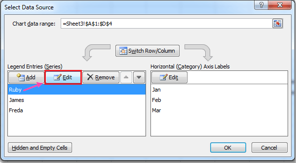
4. หลังจากกำหนดชื่อและสูตรสำหรับข้อมูลแต่ละคอลัมน์แล้วให้คลิกขวาที่คอลัมน์ใดก็ได้ในแผนภูมิของคุณแล้วเลือก เลือกข้อมูลดูภาพหน้าจอ:

เอกสารอัปเดตแผนภูมิ8

5. ใน เลือกแหล่งข้อมูล กล่องโต้ตอบจาก รายการในตำนาน (ซีรี่ส์) คลิกที่ ทับทิม และจากนั้นคลิก Edit ในปุ่มที่โผล่ออกมา แก้ไขซีรี่ส์ กล่องโต้ตอบป้อน = Sheet3! Ruby ภายใต้ ค่าชุด ดูภาพหน้าจอ:

เอกสารอัปเดตแผนภูมิ9
-1
เอกสารอัปเดตแผนภูมิ10

6. จากนั้นคลิก OK เพื่อกลับไปที่ เลือกแหล่งข้อมูล ทำซ้ำขั้นตอนที่ 5 เพื่ออัปเดตชุดข้อมูลที่เหลือเพื่อแสดงช่วงไดนามิก:

  • James: Series values: = Sheet3! James;
  • Freda: ค่าชุด: = Sheet3! Freda

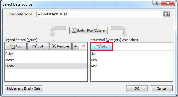
7. หลังจากตั้งค่าข้อมูลด้านซ้ายตอนนี้คุณต้องคลิก Edit ใต้ปุ่ม ป้ายกำกับแกนแนวนอน (หมวดหมู่) เพื่อตั้งค่าตัวเลือกนี้โปรดดูภาพหน้าจอ:

เอกสารอัปเดตแผนภูมิ11
-1
เอกสารอัปเดตแผนภูมิ12

8. จากนั้นคลิก OK > OK เพื่อปิด เลือกแหล่งข้อมูล หลังจากเสร็จสิ้นขั้นตอนเหล่านี้คุณจะพบว่าแผนภูมิจะอัปเดตโดยอัตโนมัติเมื่อคุณเพิ่มข้อมูลใหม่ลงในแผ่นงาน

เอกสารอัปเดตแผนภูมิ13

หมายเหตุ:

  • 1. คุณต้องป้อนข้อมูลใหม่ในลักษณะที่ต่อเนื่องกันหากคุณข้ามแถววิธีนี้จะไม่ได้ผลตามที่คาดไว้
  • 2. หากคุณป้อนข้อมูลคอลัมน์ใหม่วิธีนี้จะไม่มีผล

เคล็ดลับถ้าคุณต้องการส่งออกเนื้อหาช่วงจากแผ่นงานไปยังกราฟิกอย่างรวดเร็วโปรดลองใช้ Kutools for Excel's ช่วงการส่งออกเป็นกราฟิก ดังที่แสดงในภาพหน้าจอต่อไปนี้ มันทำงานเต็มรูปแบบโดยไม่มีข้อ จำกัด ใน [โมดูล 745} วัน โปรดดาวน์โหลดและทดลองใช้ฟรีทันที

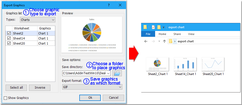
ส่งออกกราฟิก (รูปภาพ / แผนภูมิ / รูปร่าง / ทุกประเภท) จากสมุดงานไปยังโฟลเดอร์เป็น Gif / Tif / PNG / JPEG

หากมีกราฟิกหลายประเภทในสมุดงานและคุณต้องการส่งออกแผนภูมิทั้งหมดในแผ่นงานไปยังโฟลเดอร์เป็น gif ของรูปภาพประเภทอื่นคุณสามารถใช้ Kutools for Excel's Export Graphics utilty ซึ่งต้องใช้เพียง 3 ขั้นตอนในการจัดการสิ่งนี้ งาน. คลิกเพื่อทดลองใช้งานฟรี 30 วันเต็มรูปแบบ!
กราฟิกการส่งออก doc
 
Kutools for Excel: มีโปรแกรมเสริม Excel ที่มีประโยชน์มากกว่า 300 รายการให้ทดลองใช้ฟรีโดยไม่มีข้อ จำกัด ใน 30 วัน

บทความที่เกี่ยวข้อง:

วิธีเพิ่มเส้นค่าเฉลี่ยแนวนอนลงในแผนภูมิใน Excel

วิธีสร้างแผนภูมิรวมและเพิ่มแกนทุติยภูมิใน Excel

สุดยอดเครื่องมือเพิ่มผลผลิตในสำนักงาน

🤖 Kutools AI ผู้ช่วย: ปฏิวัติการวิเคราะห์ข้อมูลโดยยึดตาม: การดำเนินการที่ชาญฉลาด   |  สร้างรหัส  |  สร้างสูตรที่กำหนดเอง  |  วิเคราะห์ข้อมูลและสร้างแผนภูมิ  |  เรียกใช้ฟังก์ชัน Kutools...
คุณสมบัติยอดนิยม: ค้นหา เน้น หรือระบุรายการที่ซ้ำกัน   |  ลบแถวว่าง   |  รวมคอลัมน์หรือเซลล์โดยไม่สูญเสียข้อมูล   |   รอบโดยไม่มีสูตร ...
การค้นหาขั้นสูง: VLookup หลายเกณฑ์    VLookup หลายค่า  |   VLookup ข้ามหลายแผ่น   |   การค้นหาที่ไม่ชัดเจน ....
รายการแบบเลื่อนลงขั้นสูง: สร้างรายการแบบหล่นลงอย่างรวดเร็ว   |  รายการแบบหล่นลงขึ้นอยู่กับ   |  เลือกหลายรายการแบบหล่นลง ....
ผู้จัดการคอลัมน์: เพิ่มจำนวนคอลัมน์เฉพาะ  |  ย้ายคอลัมน์  |  สลับสถานะการมองเห็นของคอลัมน์ที่ซ่อนอยู่  |  เปรียบเทียบช่วงและคอลัมน์ ...
คุณสมบัติเด่น: กริดโฟกัส   |  มุมมองการออกแบบ   |   บาร์สูตรใหญ่    สมุดงานและตัวจัดการชีต   |  ห้องสมุดทรัพยากร (ข้อความอัตโนมัติ)   |  เลือกวันที่   |  รวมแผ่นงาน   |  เข้ารหัส/ถอดรหัสเซลล์    ส่งอีเมลตามรายการ   |  ซุปเปอร์ฟิลเตอร์   |   ตัวกรองพิเศษ (กรองตัวหนา/ตัวเอียง/ขีดทับ...) ...
ชุดเครื่องมือ 15 อันดับแรก12 ข้อความ เครื่องมือ (เพิ่มข้อความ, ลบอักขระ, ... )   |   50 + แผนภูมิ ประเภท (แผนภูมิ Gantt, ... )   |   40+ ใช้งานได้จริง สูตร (คำนวณอายุตามวันเกิด, ... )   |   19 การแทรก เครื่องมือ (ใส่ QR Code, แทรกรูปภาพจากเส้นทาง, ... )   |   12 การแปลง เครื่องมือ (ตัวเลขเป็นคำ, การแปลงสกุลเงิน, ... )   |   7 ผสานและแยก เครื่องมือ (แถวรวมขั้นสูง, แยกเซลล์, ... )   |   ... และอื่น ๆ

เพิ่มพูนทักษะ Excel ของคุณด้วย Kutools สำหรับ Excel และสัมผัสประสิทธิภาพอย่างที่ไม่เคยมีมาก่อน Kutools สำหรับ Excel เสนอคุณสมบัติขั้นสูงมากกว่า 300 รายการเพื่อเพิ่มประสิทธิภาพและประหยัดเวลา  คลิกที่นี่เพื่อรับคุณสมบัติที่คุณต้องการมากที่สุด...

รายละเอียด


แท็บ Office นำอินเทอร์เฟซแบบแท็บมาที่ Office และทำให้งานของคุณง่ายขึ้นมาก

  • เปิดใช้งานการแก้ไขและอ่านแบบแท็บใน Word, Excel, PowerPoint, ผู้จัดพิมพ์, Access, Visio และโครงการ
  • เปิดและสร้างเอกสารหลายรายการในแท็บใหม่ของหน้าต่างเดียวกันแทนที่จะเป็นในหน้าต่างใหม่
  • เพิ่มประสิทธิภาพการทำงานของคุณ 50% และลดการคลิกเมาส์หลายร้อยครั้งให้คุณทุกวัน!
Comments (21)
No ratings yet. Be the first to rate!
This comment was minimized by the moderator on the site
Good afternoon, I have a table for calculating points, on another sheet. is needed on another sheet so that there is an automatic sorting of commands by place
This comment was minimized by the moderator on the site
What if the months were in the columns and you had data series in the rows, how would you do the formula then?
This comment was minimized by the moderator on the site
Doesnt work or not applicable. My chart already refers to the correct data automatically... data is directed to table columns. The problem is the GRAPH wont update.
This comment was minimized by the moderator on the site
HI,
This trick doesnt work if you want to add new columns. This trick is for fixed columns. What if there is a data yearwise in columns and every year a new year column is added so how will it get added to the chart ??

Any idea you can suggest ??

Cheers,

Mufaddal
This comment was minimized by the moderator on the site
when I type in cell any no. like - 210 it reflect as = 2.10 , no formula is taking place why? any no. shows devide by 100 as I mentioned , decimal comes automatically how to resolve this ?
This comment was minimized by the moderator on the site
It works well! Thank you! One question: what if my drop down list is not on the same sheet with the "table" where i have datas? how can I modify the function?
This comment was minimized by the moderator on the site
Thanks for the message. But I do not get your question clearly, why don't you upload a screenshot of your problem for me to understand easily? More description, easier to understand. Thank u.
This comment was minimized by the moderator on the site
did you manage to solve this issue? having same issue at the moment
This comment was minimized by the moderator on the site
Airtel mobile Bill Payment
This comment was minimized by the moderator on the site
A chart's ranges can depend on names or not. If a chart range depends on, say A1:E5, and you insert a row at row 3, and a column at column C, the chart will automatically depend on A1:F6. Similarly, if you have a name defined as A1:E5, whether you use it as a chart's range or not, and you insert a column and row at C3, the name's definition will expand to A1:F6. But in either case, if you insert a column and A or E (the endpoints), or a row at 1 or 5, the behavior isn't so well defined: maybe the chart range or name's definition will expand; maybe it won't. To answer Melissa, you'd have to insert rows or columns before or to the left of the chart range. I think it's better to use names, because names can be defined using formulas that involve OFFSET, COUNT, INDEX, MATCH, whatever else. So the better answer to Melissa is to define a name for one cell, namely the last of the eight columns or rows, then define the name in term of an OFFSET from that cell: OFFSET(cell,-8,-8,8,8) to go back and up eight cells and use an 8x8 range.
This comment was minimized by the moderator on the site
Great reminder as I don't do these kind of chart functions that often. As an improvement you could mention how to edit defined names in the name manager but I'm not sure if the editing actually enables the function of the adding rows to work completely
This comment was minimized by the moderator on the site
You can define chart ranges with names or not -- in either case if you physically insert rows or columns in the middle of a range, it automatically expands. I think it's best to use names for charts and lots of other things, because you can define names as formulas, not just straight ranges. You must use OFFSET (which resizes too), because that returns a range, but its parameters, which are numbers, can be specified with formulas that use INDEX, MATCH, COUNT, SUM, VLOOKUP, any crazy formula you want. Melissa, that's the best way to handle your situation: give a name to one bookmark cell, then define another name to be offset from that -8 rows or columns, and resize it 8 rows or columns.
This comment was minimized by the moderator on the site
Hi there, thank you so much for this tutorial. I am just wondering, how to apply this method to the data that updated in the column not in the row? is there any additional changes that I need to do besides offset formula? thank you.
There are no comments posted here yet
Load More
Please leave your comments in English
Posting as Guest
×
Rate this post:
0   Characters
Suggested Locations