ไปยังเนื้อหาหลัก

วิธีส่งคืนค่าที่ตรงกันหลายค่าตามเกณฑ์หนึ่งหรือหลายเกณฑ์ใน Excel

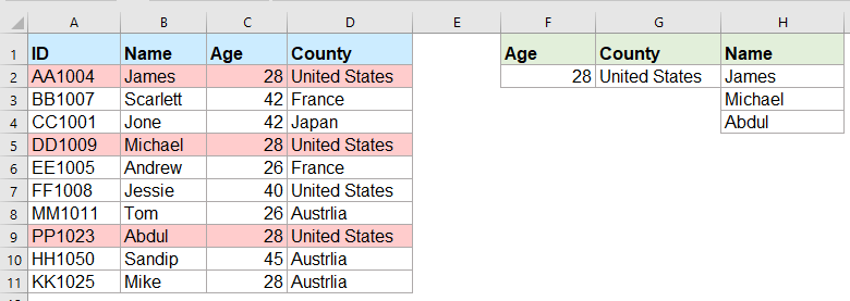
โดยปกติการค้นหาค่าเฉพาะและส่งคืนรายการที่ตรงกันนั้นเป็นเรื่องง่ายสำหรับพวกเราส่วนใหญ่โดยใช้ฟังก์ชัน VLOOKUP แต่คุณเคยพยายามส่งคืนค่าที่ตรงกันหลายค่าตามเกณฑ์อย่างน้อยหนึ่งเกณฑ์ตามภาพหน้าจอต่อไปนี้หรือไม่? ในบทความนี้ฉันจะแนะนำสูตรสำหรับแก้งานที่ซับซ้อนนี้ใน Excel

ส่งคืนค่าที่ตรงกันหลายค่าตามเกณฑ์หนึ่งหรือหลายเกณฑ์ด้วยสูตรอาร์เรย์


ส่งคืนค่าที่ตรงกันหลายค่าตามเกณฑ์หนึ่งหรือหลายเกณฑ์ด้วยสูตรอาร์เรย์

ตัวอย่างเช่นฉันต้องการแยกชื่อทั้งหมดที่มีอายุ 28 ปีและมาจากสหรัฐอเมริกาโปรดใช้สูตรต่อไปนี้:

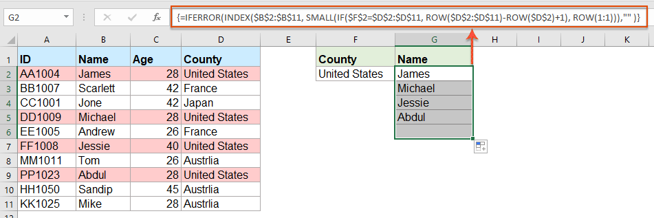
1. คัดลอกหรือป้อนสูตรด้านล่างลงในเซลล์ว่างที่คุณต้องการค้นหาผลลัพธ์:

=INDEX($B$2:$B$11, SMALL(IF(COUNTIF($F$2, $C$2:$C$11)*COUNTIF($G$2, $D$2:$D$11), ROW($A$2:$D$11)-MIN(ROW($A$2:$D$11))+1), ROW(A1)), COLUMN(A1))

หมายเหตุ: ในสูตรข้างต้น B2: B11 คือคอลัมน์ที่ส่งคืนค่าที่ตรงกัน F2, C2: C11 เป็นเงื่อนไขแรกและข้อมูลคอลัมน์ที่มีเงื่อนไขแรก G2, D2: D11 เป็นเงื่อนไขที่สองและข้อมูลคอลัมน์ที่มีเงื่อนไขนี้โปรดเปลี่ยนตามความต้องการของคุณ

2. จากนั้นกด Ctrl + Shift + Enter เพื่อรับผลลัพธ์การจับคู่แรกจากนั้นเลือกเซลล์สูตรแรกแล้วลากที่จับเติมลงไปที่เซลล์จนกว่าค่าข้อผิดพลาดจะปรากฏขึ้นตอนนี้ค่าที่ตรงกันทั้งหมดจะถูกส่งกลับตามภาพด้านล่างที่แสดง:

เคล็ดลับ: หากคุณต้องการส่งคืนค่าที่ตรงกันทั้งหมดตามเงื่อนไขเดียวโปรดใช้สูตรอาร์เรย์ด้านล่าง:

=IFERROR(INDEX($B$2:$B$11, SMALL(IF($F$2=$D$2:$D$11, ROW($D$2:$D$11)-ROW($D$2)+1), ROW(1:1))),"" )


บทความที่เกี่ยวข้องเพิ่มเติม:

  • ส่งคืนค่าการค้นหาหลายค่าในเซลล์เดียวที่คั่นด้วยจุลภาค
  • ใน Excel เราสามารถใช้ฟังก์ชัน VLOOKUP เพื่อส่งคืนค่าที่ตรงกันแรกจากเซลล์ตาราง แต่บางครั้งเราจำเป็นต้องแยกค่าที่ตรงกันทั้งหมดแล้วคั่นด้วยตัวคั่นเฉพาะเช่นลูกน้ำเส้นประ ฯลฯ ... เป็นค่าเดียว เซลล์ดังภาพหน้าจอต่อไปนี้ที่แสดง เราจะรับและส่งคืนค่าการค้นหาหลายค่าในเซลล์ที่คั่นด้วยจุลภาคหนึ่งเซลล์ใน Excel ได้อย่างไร
  • Vlookup และส่งคืนค่าที่ตรงกันหลายค่าพร้อมกันใน Google Sheet
  • ฟังก์ชัน Vlookup ปกติใน Google ชีตสามารถช่วยให้คุณค้นหาและส่งคืนค่าที่ตรงกันแรกตามข้อมูลที่กำหนด แต่บางครั้งคุณอาจต้อง vlookup และคืนค่าที่ตรงกันทั้งหมดตามภาพหน้าจอต่อไปนี้ คุณมีวิธีที่ง่ายและดีในการแก้ปัญหานี้ใน Google ชีตหรือไม่?
  • Vlookup และส่งคืนค่าหลายค่าจากรายการแบบหล่นลง
  • ใน Excel คุณจะ vlookup และส่งคืนค่าที่เกี่ยวข้องหลายค่าจากรายการแบบเลื่อนลงได้อย่างไรซึ่งหมายความว่าเมื่อคุณเลือกหนึ่งรายการจากรายการแบบหล่นลงค่าสัมพัทธ์ทั้งหมดจะแสดงพร้อมกันตามภาพหน้าจอต่อไปนี้ บทความนี้ผมจะแนะนำวิธีการแก้ปัญหาทีละขั้นตอน
  • Vlookup และส่งคืนค่าหลายค่าในแนวตั้งใน Excel
  • โดยปกติคุณสามารถใช้ฟังก์ชัน Vlookup เพื่อรับค่าแรกที่สอดคล้องกัน แต่บางครั้งคุณต้องการส่งคืนระเบียนที่ตรงกันทั้งหมดตามเกณฑ์เฉพาะ บทความนี้ฉันจะพูดถึงวิธี vlookup และส่งคืนค่าที่ตรงกันทั้งหมดในแนวตั้งแนวนอนหรือในเซลล์เดียว
  • Vlookup และส่งคืนข้อมูลที่ตรงกันระหว่างค่าสองค่าใน Excel
  • ใน Excel เราสามารถใช้ฟังก์ชัน Vlookup ปกติเพื่อรับค่าที่สอดคล้องกันตามข้อมูลที่กำหนด แต่บางครั้งเราต้องการ vlookup และส่งคืนค่าที่ตรงกันระหว่างสองค่าตามภาพหน้าจอต่อไปนี้คุณจะจัดการกับงานนี้ใน Excel ได้อย่างไร?


เครื่องมือเพิ่มประสิทธิภาพการทำงานในสำนักงานที่ดีที่สุด

Kutools สำหรับ Excel แก้ปัญหาส่วนใหญ่ของคุณและเพิ่มผลผลิตของคุณได้ถึง 80%

  • ซุปเปอร์ฟอร์มูล่าบาร์ (แก้ไขข้อความและสูตรหลายบรรทัดได้อย่างง่ายดาย); การอ่านเค้าโครง (อ่านและแก้ไขเซลล์จำนวนมากได้อย่างง่ายดาย); วางลงในช่วงที่กรองแล้ว...
  • ผสานเซลล์ / แถว / คอลัมน์ และการเก็บรักษาข้อมูล แยกเนื้อหาของเซลล์ รวมแถวที่ซ้ำกันและผลรวม / ค่าเฉลี่ย... ป้องกันเซลล์ซ้ำ; เปรียบเทียบช่วง...
  • เลือกซ้ำหรือไม่ซ้ำ แถว; เลือกแถวว่าง (เซลล์ทั้งหมดว่างเปล่า); Super Find และ Fuzzy Find ในสมุดงานจำนวนมาก สุ่มเลือก ...
  • สำเนาถูกต้อง หลายเซลล์โดยไม่เปลี่ยนการอ้างอิงสูตร สร้างการอ้างอิงอัตโนมัติ ถึงหลายแผ่น ใส่สัญลักษณ์แสดงหัวข้อย่อย, กล่องกาเครื่องหมายและอื่น ๆ ...
  • แทรกสูตรที่ชื่นชอบและรวดเร็ว, ช่วงแผนภูมิและรูปภาพ; เข้ารหัสเซลล์ ด้วยรหัสผ่าน; สร้างรายชื่อผู้รับจดหมาย และส่งอีเมล ...
  • แยกข้อความ, เพิ่มข้อความ, ลบตามตำแหน่ง, ลบ Space; สร้างและพิมพ์ผลรวมย่อยของเพจ แปลงระหว่างเนื้อหาของเซลล์และความคิดเห็น...
  • ซุปเปอร์ฟิลเตอร์ (บันทึกและใช้โครงร่างตัวกรองกับแผ่นงานอื่น ๆ ); การเรียงลำดับขั้นสูง ตามเดือน / สัปดาห์ / วันความถี่และอื่น ๆ ตัวกรองพิเศษ โดยตัวหนาตัวเอียง ...
  • รวมสมุดงานและแผ่นงาน; ผสานตารางตามคอลัมน์สำคัญ แยกข้อมูลออกเป็นหลายแผ่น; Batch แปลง xls, xlsx และ PDF...
  • การจัดกลุ่มตาราง Pivot ตาม จำนวนสัปดาห์วันในสัปดาห์และอื่น ๆ ... แสดงปลดล็อกเซลล์ที่ถูกล็อก ด้วยสีที่ต่างกัน เน้นเซลล์ที่มีสูตร / ชื่อ...
kte แท็บ 201905
  • เปิดใช้งานการแก้ไขและอ่านแบบแท็บใน Word, Excel, PowerPoint, ผู้จัดพิมพ์, Access, Visio และโครงการ
  • เปิดและสร้างเอกสารหลายรายการในแท็บใหม่ของหน้าต่างเดียวกันแทนที่จะเป็นในหน้าต่างใหม่
  • เพิ่มประสิทธิภาพการทำงานของคุณ 50% และลดการคลิกเมาส์หลายร้อยครั้งให้คุณทุกวัน!
ด้านล่าง officetab


Comments (25)
No ratings yet. Be the first to rate!
This comment was minimized by the moderator on the site
Hi, if there are duplicate values (e.g. two adams), how do i make sure that it only returns 1 adam and not 2?
This comment was minimized by the moderator on the site
Hello, Bobby,
To extract only unique matching values, you should apply the below formula:
After pasting the formula, please press Ctrl + Shift + Enter keys together to get the correct result.
=IFERROR(INDEX($B$2:$B$5, MATCH(0, COUNTIF(H1:$H$1, $B$2:$B$5)+IF($D$2:$D$5<>$G$2, 1, 0)+IF($C$2:$C$5<>$F$2, 1, 0), 0)), "")

Please have a try, hope it can help you!
This comment was minimized by the moderator on the site
Hi,

Thanks for posting these examples.
I'm trying to implement this in my own sheet, but don't get it to work (maybe because I'm using an europe version of excel)?

I want to get the dates of the days that I had my shifts or that I have worked 'some' (>0) hours for a client.

So in I3 is the name and in J3 the month. K3 and L3 are the shifts (1 is worked) and hours (don't know how to set this, should be more than zero)

My expected results are in:
Shifts: I7 and I8
hours: J7

So I worked more than 0 hours for 'person 2' in oktober on 3-10-2022
had shifts for person 2 on '10-10-2022' and 28-10-2022

When I add '=INDEX($B$2:$B$11, SMALL(IF(COUNTIF($F$2, $C$2:$C$11)*COUNTIF($G$2, $D$2:$D$11), ROW($A$2:$D$11)-MIN(ROW($A$2:$D$11))+1), ROW(A1)), COLUMN(A1))' in my excel sheet, it doesn't allow the comma between the different parts of the formula.
So I need to change them to ';'.
But when I try it it always says: '#NAME?'

So can someone help me with this?

Kind regards,

Bas
[img]https://drive.google.com/file/d/1iIPQKuj_PNhqWyWlwJ4IQTqGNEd6B9Hw/view?usp=share_link[/img]
This comment was minimized by the moderator on the site
Hi,

First, thank you for sharing!

Can you please provide a solution to the case below:

I have 3 columns (A: Containing reference information, B: Containing information to be searched, C: Search result)

Image url is provided below

https://ibb.co/VHCd09K

Column A-------------------------Column B------------Column C
File Name-------------------------Name----------------File Name, Document Name, Element Name, Name
Changed Element-----------------Element--------------Changed Element, Element Name, Element ID
Column Location
Document Name
Element Name
Name
Category
Warranty
Slope
Element ID

What I need is to search in column A for any partial match with cell B2 (Name) or B3 (Element) and get the result in one cell,

Thank you, Behzad
This comment was minimized by the moderator on the site
Hello, Behzad
Maybe the below User Defined Function can help you.
Public Function ConcatPartLookUp(rngInput As Range, rngSource As Range, Optional strDelimiter As String, Optional blCaseSensitive)
Dim rng As Range
If strDelimiter = "" Then strDelimiter = ","
If IsMissing(blCaseSensitive) Then
    blCaseSensitive = False
Else
    blCaseSensitive = True
End If
For Each rng In rngSource
    If blCaseSensitive Then
        If InStr(1, rng.Value, rngInput.Value, vbBinaryCompare) > 0 Then ConcatPartLookUp = ConcatPartLookUp & strDelimiter & rng.Value
    Else
        If InStr(1, rng.Value, rngInput.Value, vbTextCompare) > 0 Then ConcatPartLookUp = ConcatPartLookUp & strDelimiter & rng.Value
    End If
Next
If Len(ConcatPartLookUp) > 0 Then ConcatPartLookUp = Mid(ConcatPartLookUp, 2, Len(ConcatPartLookUp))
End Function


After copying and pasting this code, and then use this formula:=ConcatPartLookUp(B2,$A$2:$A$8) to get the result you need.
Please have a try, hope it can help you!
This comment was minimized by the moderator on the site
Heyi, thank you for the formula. It worked for "fixed" values / text as criterias. However, one of the criterias i'm trying to use is a condition (values <>0 ), but does not work the described formula. Do you guys know what should i change to adapt the formula so I can have a condition as one of the criterias, please?

Best,

João
This comment was minimized by the moderator on the site
Hello, Marcus
To solve your problem, please view this article:
https://www.extendoffice.com/documents/excel/6393-excel-vlookup-function.html#b3-2
There are some detailed explanations of this task. You just need to change the criteira to your own.
Thank you!
This comment was minimized by the moderator on the site
Hi,

if in cell H1 i write "Name" and wanted to link that with the formula, how would that work?
Then I could write "ID" in cell H1 and would automatically get as a result: AA1004; DD1009; PP1023 (for the first formula)

Thank you in advance!
This comment was minimized by the moderator on the site
Hello, Marie
Sorry, i can't get the point of your first problem, could you explain your problem more clearly and detailedly? Or you can insert a screenshot here to describe your problem.
As for the second question, you just need to change the cell reference as this:
=INDEX($A$2:$A$11, SMALL(IF(COUNTIF($F$2, $C$2:$C$11)*COUNTIF($G$2, $D$2:$D$11), ROW($A$2:$D$11)-MIN(ROW($A$2:$D$11))+1), ROW(A1)), COLUMN(A1))

Remeber to press Ctrl + Shift + Enter keys together.
Please try, hope it can help you!
This comment was minimized by the moderator on the site
Hello,
what would be needed to expand the first formula in the following case:
Some IDs are Blank (e.g. cell A5 is blank) and I would like an additional condition outputting lines only when the IDs are not blank. (So the output should then be James and Abdul.
Thanks!
This comment was minimized by the moderator on the site
Hello, Jo,
To solve your problem, please apply the below formula:
=INDEX($B$2:$B$11, SMALL(IF(COUNTIF($F$2, $C$2:$C$11)*COUNTIF($G$2, $D$2:$D$11)*($A$2:$A$11<>0), ROW($A$2:$D$11)-MIN(ROW($A$2:$D$11))+1), ROW(A1)), COLUMN(A1))

Please have a ry, hope it can help you!
This comment was minimized by the moderator on the site
hello,
ive tried using the formula and it either generates a value of 0 or the image attached
This comment was minimized by the moderator on the site
Hello, Milku
Your screenshot showed WPS software of MAC version, so I am not sure whether our formula is available.
I uploaded an Excel file to here, you can try to see if it can calculate correctly in you environment.
Thank you!
This comment was minimized by the moderator on the site
When I use the second formula and drag down, nothing appears. The formula result (fx) says it should be returning something but it is blank. How do I correct this?
This comment was minimized by the moderator on the site
Hello Alysia,

Glad to help. I tried the second formula in the article and drag the formula down, the rest of results were returned. I think there may be two reasons for your problem. First, maybe you forget to press Ctrl + Shift + Enter keys to enter the formula. Second, the matching result is only one, so no other results are not returned. Please have a check.

Sincerely,
Mandy
This comment was minimized by the moderator on the site
Hi,

I was wondering if it at all possible to enter a 2nd criteria but from the same range as the 1st criteria,

For example with the used example above i would like to search for the names of people from both America and France So cell F3 would have France, Scarlett & Andrew would also populate in the list in Column G

Thank you for assistance in advance.
This comment was minimized by the moderator on the site
Hello Nick,

Glad to help. If you want to get the names of people from both America and France, I advise you to use our formula twice to get the result. Please see the screenshot, In F2 and G2 are values "United States" and "France". Apply formula =IFERROR(INDEX($B$2:$B$11, SMALL(IF($F$2=$D$2:$D$11, ROW($D$2:$D$11)-ROW($D$2)+1), ROW(1:1))),"" ) to get the results for America. And apply formula =IFERROR(INDEX($B$2:$B$11, SMALL(IF($G$2=$D$2:$D$11, ROW($D$2:$D$11)-ROW($D$2)+1), ROW(1:1))),"" ) to get the results for France. It's simple. Please have a try.

Sincerely,
Mandy
This comment was minimized by the moderator on the site
In the first example, what change to the formula would be needed to return everyone who was less than 28 years old?
There are no comments posted here yet
Load More
Please leave your comments in English
Posting as Guest
×
Rate this post:
0   Characters
Suggested Locations