วิธี vlookup และส่งคืนสีพื้นหลังพร้อมกับค่าการค้นหาใน Excel

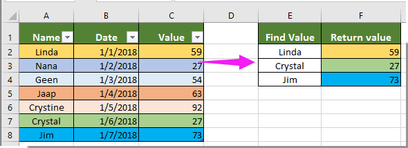
สมมติว่าคุณมีตารางตามภาพด้านล่างที่แสดง ตอนนี้คุณต้องการตรวจสอบว่าค่าที่ระบุอยู่ในคอลัมน์ A หรือไม่จากนั้นส่งคืนค่าที่เกี่ยวข้องพร้อมกับสีพื้นหลังในคอลัมน์ C จะบรรลุได้อย่างไร วิธีการในบทความสามารถช่วยคุณแก้ปัญหาได้

Vlookup และส่งคืนสีพื้นหลังพร้อมค่าการค้นหาโดยฟังก์ชันที่ผู้ใช้กำหนดเอง

Vlookup และส่งคืนสีพื้นหลังพร้อมค่าการค้นหาโดยฟังก์ชันที่ผู้ใช้กำหนดเอง

อัศจรรย์! การใช้แท็บที่มีประสิทธิภาพใน Excel เช่น Chrome, Edge, Firefox และ Safari!
ประหยัดเวลา 50% และลดการคลิกเมาส์หลายพันครั้งให้คุณทุกวัน!

โปรดทำดังนี้เพื่อค้นหาค่าและส่งคืนค่าที่เกี่ยวข้องพร้อมกับสีพื้นหลังใน Excel

1. ในแผ่นงานมีค่าที่คุณต้องการ vlookup ให้คลิกขวาที่แท็บแผ่นงานแล้วเลือก ดูรหัส จากเมนูบริบท ดูภาพหน้าจอ:

2. ในการเปิด Microsoft Visual Basic สำหรับแอปพลิเคชัน โปรดคัดลอกโค้ด VBA ด้านล่างลงในหน้าต่างรหัส

รหัส VBA 1: Vlookup และส่งคืนสีพื้นหลังพร้อมค่าการค้นหา

Sub Worksheet_Change(ByVal Target As Range)
    Dim I As Long
    Dim xKeys As Long
    Dim xDicStr As String
    On Error Resume Next
    Application.ScreenUpdating = False
    xKeys = UBound(xDic.Keys)
    If xKeys >= 0 Then
        For I = 0 To UBound(xDic.Keys)
            xDicStr = xDic.Items(I)
            If xDicStr <> "" Then
                Range(xDic.Keys(I)).Interior.Color = _
                Range(xDic.Items(I)).Interior.Color
            Else
                Range(xDic.Keys(I)).Interior.Color = xlNone
            End If
        Next
        Set xDic = Nothing
    End If
    Application.ScreenUpdating = True
End Sub

3 จากนั้นคลิก สิ่งที่ใส่เข้าไป > โมดูลแล้วคัดลอกโค้ด VBA 2 ด้านล่างลงในหน้าต่างโมดูล

รหัส VBA 2: Vlookup และส่งคืนสีพื้นหลังพร้อมค่าการค้นหา

Public xDic As New Dictionary
Function LookupKeepColor (ByRef FndValue, ByRef LookupRng As Range, ByRef xCol As Long)
    Dim xFindCell As Range
    On Error Resume Next
    Set xFindCell = LookupRng.Find(FndValue, , xlValues, xlWhole)
    If xFindCell Is Nothing Then
        LookupKeepColor = ""
        xDic.Add Application.Caller.Address, ""
    Else
        LookupKeepColor = xFindCell.Offset(0, xCol - 1).Value
        xDic.Add Application.Caller.Address, xFindCell.Offset(0, xCol - 1).Address
    End If
End Function

4. หลังจากใส่รหัสทั้งสองแล้วคลิก เครื่องมือ > อ้างอิง. จากนั้นตรวจสอบไฟล์ รันไทม์ Microsoft Script กล่องใน เอกสารอ้างอิง - VBAProject กล่องโต้ตอบ ดูภาพหน้าจอ:

5 กด อื่น ๆ + Q ปุ่มเพื่อออกจากไฟล์ Microsoft Visual Basic สำหรับแอปพลิเคชัน หน้าต่างและกลับไปที่แผ่นงาน

6. เลือกเซลล์ว่างที่อยู่ติดกับค่าการค้นหาจากนั้นป้อนสูตร =LookupKeepColor(E2,$A$1:$C$8,3) ลงในแถบสูตรแล้วกดปุ่ม Enter

หมายเหตุ: ในสูตร E2 มีค่าที่คุณจะค้นหา $ ก $ 1: $ C $ 8 คือช่วงของตารางและตัวเลข 3 หมายความว่าค่าที่สอดคล้องกันที่คุณจะส่งคืนจะอยู่ในคอลัมน์ที่สามของตาราง โปรดเปลี่ยนตามที่คุณต้องการ

7. เลือกเซลล์ผลลัพธ์แรกจากนั้นลาก Fill Handle ลงเพื่อให้ได้ผลลัพธ์ทั้งหมดพร้อมกับสีพื้นหลัง ดูภาพหน้าจอ

บทความที่เกี่ยวข้อง:

• วิธีคัดลอกการจัดรูปแบบแหล่งที่มาของเซลล์การค้นหาเมื่อใช้ Vlookup ใน Excel
• วิธี vlookup และรูปแบบวันที่ส่งคืนแทนตัวเลขใน Excel
• วิธีใช้ vlookup และ sum ใน Excel
• วิธีการส่งคืนค่า vlookup ในเซลล์ที่อยู่ติดกันหรือถัดไปใน Excel
• วิธีการ vlookup ค่าและส่งคืนจริงหรือเท็จ / ใช่หรือไม่ใช่ใน Excel?

สุดยอดเครื่องมือเพิ่มผลผลิตในสำนักงาน

🤖	Kutools AI ผู้ช่วย: ปฏิวัติการวิเคราะห์ข้อมูลโดยยึดตาม: การดำเนินการที่ชาญฉลาด   |  สร้างรหัส  |  สร้างสูตรที่กำหนดเอง  |  วิเคราะห์ข้อมูลและสร้างแผนภูมิ  |  เรียกใช้ฟังก์ชัน Kutools...
	คุณสมบัติยอดนิยม: ค้นหา เน้น หรือระบุรายการที่ซ้ำกัน   |  ลบแถวว่าง   |  รวมคอลัมน์หรือเซลล์โดยไม่สูญเสียข้อมูล   |   รอบโดยไม่มีสูตร ...
	การค้นหาขั้นสูง: VLookup หลายเกณฑ์  |   VLookup หลายค่า  |   VLookup ข้ามหลายแผ่น   |   การค้นหาที่ไม่ชัดเจน ....
	รายการแบบเลื่อนลงขั้นสูง: สร้างรายการแบบหล่นลงอย่างรวดเร็ว   |  รายการแบบหล่นลงขึ้นอยู่กับ   |  เลือกหลายรายการแบบหล่นลง ....
	ผู้จัดการคอลัมน์: เพิ่มจำนวนคอลัมน์เฉพาะ  |  ย้ายคอลัมน์  |  สลับสถานะการมองเห็นของคอลัมน์ที่ซ่อนอยู่  |  เปรียบเทียบช่วงและคอลัมน์ ...
	คุณสมบัติเด่น: กริดโฟกัส   |  มุมมองการออกแบบ   |   บาร์สูตรใหญ่   |  สมุดงานและตัวจัดการชีต   |  ห้องสมุดทรัพยากร (ข้อความอัตโนมัติ)   |  เลือกวันที่   |  รวมแผ่นงาน   |  เข้ารหัส/ถอดรหัสเซลล์   |  ส่งอีเมลตามรายการ   |  ซุปเปอร์ฟิลเตอร์   |   ตัวกรองพิเศษ (กรองตัวหนา/ตัวเอียง/ขีดทับ...) ...
	ชุดเครื่องมือ 15 อันดับแรก:  12 ข้อความ เครื่องมือ (เพิ่มข้อความ, ลบอักขระ, ... )   |   50 + แผนภูมิ ประเภท (แผนภูมิ Gantt, ... )   |   40+ ใช้งานได้จริง สูตร (คำนวณอายุตามวันเกิด, ... )   |   19 การแทรก เครื่องมือ (ใส่ QR Code, แทรกรูปภาพจากเส้นทาง, ... )   |   12 การแปลง เครื่องมือ (ตัวเลขเป็นคำ, การแปลงสกุลเงิน, ... )   |   7 ผสานและแยก เครื่องมือ (แถวรวมขั้นสูง, แยกเซลล์, ... )   |   ... และอื่น ๆ

เพิ่มพูนทักษะ Excel ของคุณด้วย Kutools สำหรับ Excel และสัมผัสประสิทธิภาพอย่างที่ไม่เคยมีมาก่อน Kutools สำหรับ Excel เสนอคุณสมบัติขั้นสูงมากกว่า 300 รายการเพื่อเพิ่มประสิทธิภาพและประหยัดเวลา  คลิกที่นี่เพื่อรับคุณสมบัติที่คุณต้องการมากที่สุด...

อ่านเพิ่มเติม ... ดาวน์โหลดฟรี...

---

แท็บ Office นำอินเทอร์เฟซแบบแท็บมาที่ Office และทำให้งานของคุณง่ายขึ้นมาก

• เปิดใช้งานการแก้ไขและอ่านแบบแท็บใน Word, Excel, PowerPoint, ผู้จัดพิมพ์, Access, Visio และโครงการ
• เปิดและสร้างเอกสารหลายรายการในแท็บใหม่ของหน้าต่างเดียวกันแทนที่จะเป็นในหน้าต่างใหม่
• เพิ่มประสิทธิภาพการทำงานของคุณ 50% และลดการคลิกเมาส์หลายร้อยครั้งให้คุณทุกวัน!

อ่านเพิ่มเติม ... ดาวน์โหลดฟรี...