ไปยังเนื้อหาหลัก

วิธีตรวจสอบว่าเซลล์มีค่าใดค่าหนึ่งใน Excel หรือไม่?

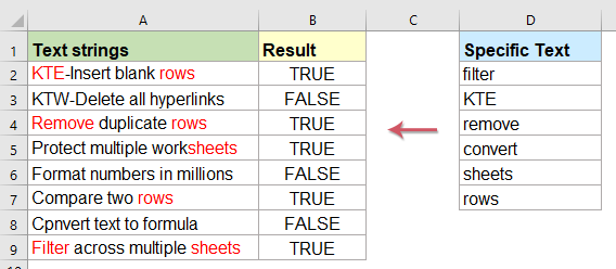
สมมติว่าคุณมีรายการสตริงข้อความในคอลัมน์ A ตอนนี้คุณต้องการทดสอบแต่ละเซลล์ว่ามีค่าใดค่าหนึ่งตามช่วงอื่น D2: D7 หากมีข้อความเฉพาะใน D2: D7 ก็จะแสดง True มิฉะนั้นจะแสดง False ตามภาพหน้าจอต่อไปนี้ บทความนี้ฉันจะพูดถึงวิธีการระบุเซลล์หากมีหลายค่าในช่วงอื่น


ตรวจสอบว่าเซลล์มีหนึ่งในหลายค่าจากรายการที่มีสูตรหรือไม่

หากต้องการตรวจสอบว่าเนื้อหาของเซลล์มีค่าข้อความใด ๆ ในช่วงอื่นหรือไม่สูตรต่อไปนี้อาจช่วยคุณได้โปรดดำเนินการดังนี้:

ป้อนสูตรด้านล่างลงในเซลล์ว่างที่คุณต้องการค้นหาผลลัพธ์เช่น B2 จากนั้นลากที่จับเติมลงไปที่เซลล์ที่คุณต้องการใช้สูตรนี้และหากเซลล์นั้นมีค่าข้อความใด ๆ ในอีกเซลล์หนึ่ง เฉพาะบางช่วงก็จะได้ True มิฉะนั้นจะได้ False ดูภาพหน้าจอ:

=SUMPRODUCT(--ISNUMBER(SEARCH($D$2:$D$7,A2)))>0

ทิปส์:

1. หากคุณต้องการใช้ "ใช่" หรือ "ไม่" เพื่อระบุผลลัพธ์โปรดใช้สูตรต่อไปนี้และคุณจะได้รับผลลัพธ์ต่อไปนี้ตามที่คุณต้องการโปรดดูภาพหน้าจอ:

=IF(SUMPRODUCT(--ISNUMBER(SEARCH($D$2:$D$6,A2))),"Yes","No")

2. ในสูตรข้างต้น D2: D7 คือช่วงข้อมูลเฉพาะที่คุณต้องการตรวจสอบเซลล์ตามและ A2 คือเซลล์ที่คุณต้องการตรวจสอบ


แสดงการจับคู่หากเซลล์มีค่าใดค่าหนึ่งจากรายการที่มีสูตร

Sotimes คุณอาจต้องการตรวจสอบว่าเซลล์มีค่าในรายการหรือไม่จากนั้นส่งคืนค่านั้นหากหลายค่าตรงกันค่าที่ตรงกันทั้งหมดในรายการจะแสดงดังภาพด้านล่างนี้คุณจะแก้ปัญหานี้ใน Excel ได้อย่างไร?

หากต้องการแสดง vaues ที่ตรงกันทั้งหมดหากเซลล์มีข้อความใดข้อความหนึ่งโปรดใช้สูตรด้านล่าง:

=TEXTJOIN(", ", TRUE, IF(COUNTIF(A2, "*"&$D$2:$D$7&"*"), $D$2:$D$7, ""))

หมายเหตุ: ในสูตรข้างต้น D2: D7 คือช่วงข้อมูลเฉพาะที่คุณต้องการตรวจสอบเซลล์ตามและ A2 คือเซลล์ที่คุณต้องการตรวจสอบ

แล้วกด Ctrl + Shift + Enter เข้าด้วยกันเพื่อให้ได้ผลลัพธ์แรกจากนั้นลากที่จับเติมลงไปที่เซลล์ที่คุณต้องการใช้สูตรนี้ดูภาพหน้าจอ:

ทิปส์:

ฟังก์ชัน TEXTJOIN ข้างต้นพร้อมใช้งานสำหรับ Excel 2019 และ Office 365 เท่านั้นหากคุณมี Excel เวอร์ชันก่อนหน้าคุณควรใช้สูตรด้านล่าง:

=IFERROR(INDEX($D$2:$D$7, SMALL(IF(COUNTIF($A2, "*"&$D$2:$D$7&"*"), MATCH(ROW($D$2:$D$7), ROW($D$2:$D$7)), ""), COLUMNS($F$1:F1))), "")

หมายเหตุ: ในสูตรข้างต้น D2: D7 คือช่วงข้อมูลเฉพาะที่คุณต้องการตรวจสอบเซลล์ตามและ A2 คือเซลล์ที่คุณต้องการตรวจสอบ

แล้วกด Ctrl + Shift + Enter คีย์เข้าด้วยกันเพื่อให้ได้ผลลัพธ์แรกจากนั้นลากเซลล์สูตรไปทางด้านขวาจนกว่าเซลล์ว่างจะปรากฏขึ้นจากนั้นลากที่จับเติมลงไปที่เซลล์อื่นและค่าที่ตรงกันทั้งหมดจะแสดงดังภาพด้านล่างที่แสดง:


เน้นการจับคู่หากเซลล์มีค่าใดค่าหนึ่งจากรายการที่มีคุณสมบัติที่มีประโยชน์

หากคุณต้องการเน้นสีแบบอักษรเฉพาะสำหรับค่าที่ตรงกันหากเซลล์มีค่าใดค่าหนึ่งจากรายการอื่นส่วนนี้ฉันจะแนะนำคุณสมบัติที่ง่าย ทำเครื่องหมายคำหลัก of Kutools สำหรับ Excelด้วยยูทิลิตี้นี้คุณสามารถไฮไลต์คำหลักหนึ่งคำขึ้นไปพร้อมกันภายในเซลล์

หมายเหตุเพื่อนำไปใช้ ทำเครื่องหมายคำหลัก ประการแรกคุณควรดาวน์โหลดไฟล์ Kutools สำหรับ Excelแล้วใช้คุณสมบัติอย่างรวดเร็วและง่ายดาย

หลังจากการติดตั้ง Kutools สำหรับ Excelโปรดดำเนินการดังนี้:

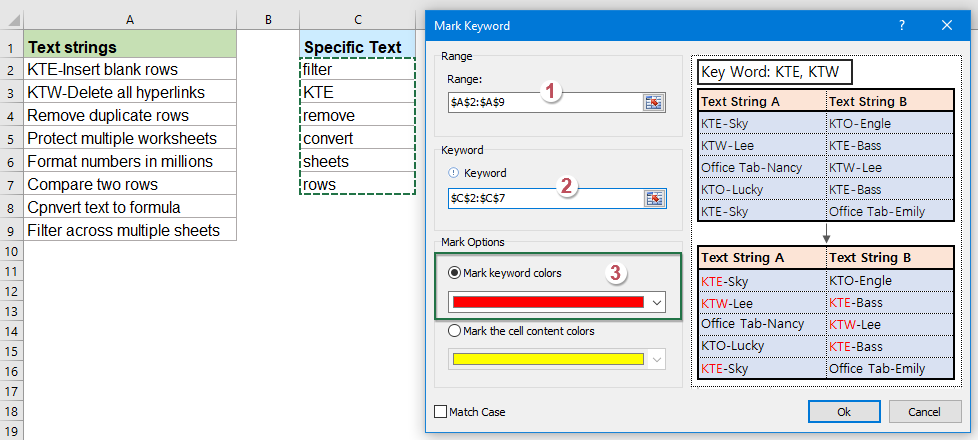
1. คลิก Kutools > ข้อความ > ทำเครื่องหมายคำหลักดูภาพหน้าจอ:

2. ใน ทำเครื่องหมายคำหลัก โปรดดำเนินการดังต่อไปนี้:

  • เลือกช่วงข้อมูลที่คุณต้องการเน้นข้อความที่ตรงกันจากไฟล์ พิสัย กล่องข้อความ;
  • เลือกเซลล์ที่มีคำสำคัญที่คุณต้องการเน้นตามคุณยังสามารถป้อนคำหลักด้วยตนเอง (คั่นด้วยลูกน้ำ) ลงใน คำหลัก กล่องข้อความ
  • สุดท้ายคุณควรระบุสีฟอนต์สำหรับไฮไลต์ข้อความด้วยกา ทำเครื่องหมายสีของคำหลัก ตัวเลือก 

3. จากนั้นคลิก Ok ปุ่มข้อความที่ตรงกันทั้งหมดได้รับการเน้นดังภาพด้านล่างที่แสดง:


บทความที่เกี่ยวข้องเพิ่มเติม:

  • เปรียบเทียบสตริงข้อความสองรายการขึ้นไปใน Excel
  • หากคุณต้องการเปรียบเทียบสตริงข้อความตั้งแต่สองสตริงขึ้นไปในแผ่นงานโดยคำนึงถึงตัวพิมพ์เล็กและใหญ่หรือไม่คำนึงถึงตัวพิมพ์เล็กและใหญ่ตามที่แสดงภาพหน้าจอต่อไปนี้บทความนี้ฉันจะพูดถึงสูตรที่มีประโยชน์สำหรับคุณในการจัดการกับงานนี้ใน Excel
  • ถ้าเซลล์มีข้อความให้แสดงใน Excel
  • หากคุณมีรายการสตริงข้อความในคอลัมน์ A และแถวของคำหลักตอนนี้คุณต้องตรวจสอบว่าคำหลักปรากฏในสตริงข้อความหรือไม่ หากคีย์เวิร์ดปรากฏในเซลล์การแสดงหากไม่มีเซลล์ว่างจะแสดงดังภาพหน้าจอต่อไปนี้
  • ค้นหาและแทนที่ค่าหลายค่าใน Excel
  • โดยปกติแล้วคุณลักษณะค้นหาและแทนที่สามารถช่วยคุณค้นหาข้อความที่ต้องการและแทนที่ด้วยข้อความอื่นได้ แต่บางครั้งคุณอาจต้องค้นหาและแทนที่ค่าหลายค่าพร้อมกัน ตัวอย่างเช่นหากต้องการแทนที่ข้อความ "Excel" ทั้งหมดเป็น "Excel 2019", "Outlook" เป็น "Outlook2019" เป็นต้นตามภาพหน้าจอด้านล่างที่แสดง บทความนี้ผมจะแนะนำสูตรสำหรับแก้งานนี้ใน Excel

สุดยอดเครื่องมือเพิ่มผลผลิตในสำนักงาน

🤖 Kutools AI ผู้ช่วย: ปฏิวัติการวิเคราะห์ข้อมูลโดยยึดตาม: การดำเนินการที่ชาญฉลาด   |  สร้างรหัส  |  สร้างสูตรที่กำหนดเอง  |  วิเคราะห์ข้อมูลและสร้างแผนภูมิ  |  เรียกใช้ฟังก์ชัน Kutools...
คุณสมบัติยอดนิยม: ค้นหา เน้น หรือระบุรายการที่ซ้ำกัน   |  ลบแถวว่าง   |  รวมคอลัมน์หรือเซลล์โดยไม่สูญเสียข้อมูล   |   รอบโดยไม่มีสูตร ...
การค้นหาขั้นสูง: VLookup หลายเกณฑ์    VLookup หลายค่า  |   VLookup ข้ามหลายแผ่น   |   การค้นหาที่ไม่ชัดเจน ....
รายการแบบเลื่อนลงขั้นสูง: สร้างรายการแบบหล่นลงอย่างรวดเร็ว   |  รายการแบบหล่นลงขึ้นอยู่กับ   |  เลือกหลายรายการแบบหล่นลง ....
ผู้จัดการคอลัมน์: เพิ่มจำนวนคอลัมน์เฉพาะ  |  ย้ายคอลัมน์  |  สลับสถานะการมองเห็นของคอลัมน์ที่ซ่อนอยู่  |  เปรียบเทียบช่วงและคอลัมน์ ...
คุณสมบัติเด่น: กริดโฟกัส   |  มุมมองการออกแบบ   |   บาร์สูตรใหญ่    สมุดงานและตัวจัดการชีต   |  ห้องสมุดทรัพยากร (ข้อความอัตโนมัติ)   |  เลือกวันที่   |  รวมแผ่นงาน   |  เข้ารหัส/ถอดรหัสเซลล์    ส่งอีเมลตามรายการ   |  ซุปเปอร์ฟิลเตอร์   |   ตัวกรองพิเศษ (กรองตัวหนา/ตัวเอียง/ขีดทับ...) ...
ชุดเครื่องมือ 15 อันดับแรก12 ข้อความ เครื่องมือ (เพิ่มข้อความ, ลบอักขระ, ... )   |   50 + แผนภูมิ ประเภท (แผนภูมิ Gantt, ... )   |   40+ ใช้งานได้จริง สูตร (คำนวณอายุตามวันเกิด, ... )   |   19 การแทรก เครื่องมือ (ใส่ QR Code, แทรกรูปภาพจากเส้นทาง, ... )   |   12 การแปลง เครื่องมือ (ตัวเลขเป็นคำ, การแปลงสกุลเงิน, ... )   |   7 ผสานและแยก เครื่องมือ (แถวรวมขั้นสูง, แยกเซลล์, ... )   |   ... และอื่น ๆ

เพิ่มพูนทักษะ Excel ของคุณด้วย Kutools สำหรับ Excel และสัมผัสประสิทธิภาพอย่างที่ไม่เคยมีมาก่อน Kutools สำหรับ Excel เสนอคุณสมบัติขั้นสูงมากกว่า 300 รายการเพื่อเพิ่มประสิทธิภาพและประหยัดเวลา  คลิกที่นี่เพื่อรับคุณสมบัติที่คุณต้องการมากที่สุด...

รายละเอียด


แท็บ Office นำอินเทอร์เฟซแบบแท็บมาที่ Office และทำให้งานของคุณง่ายขึ้นมาก

  • เปิดใช้งานการแก้ไขและอ่านแบบแท็บใน Word, Excel, PowerPoint, ผู้จัดพิมพ์, Access, Visio และโครงการ
  • เปิดและสร้างเอกสารหลายรายการในแท็บใหม่ของหน้าต่างเดียวกันแทนที่จะเป็นในหน้าต่างใหม่
  • เพิ่มประสิทธิภาพการทำงานของคุณ 50% และลดการคลิกเมาส์หลายร้อยครั้งให้คุณทุกวัน!
Comments (56)
No ratings yet. Be the first to rate!
This comment was minimized by the moderator on the site
Hello,

I have spreadsheet that have some cell with following test $5655 (BIT001), $4445 (BIT002). I would like to extract every BITxxx and display in another cell with BIT001, BIT002. I'm using MID and FIND but it work only with one BIT001 and BIT002 seems to not search. How would you do it guys?
This comment was minimized by the moderator on the site
You can use text to column > Deliminate > ("("), - I will spit the text from Open Bracket .. like BIT001), then you can remove the closing bracket with a find and replace option.
This comment was minimized by the moderator on the site
Hi all,

Any suggestions...

I have a VALUE next to the SPECIFIC TEXT column F. I need a RESULT in Column B with the VALUE next to SPECIFIC TEXT.
This comment was minimized by the moderator on the site
In option "Display the matches if cell contains one of several values from a list with formulas" I'm having issues in "Result" when the "Specific Text" values is similar to others.

For example, if I have in "Specific Text" the values 'remove' and 'remove lines', I need to get in "Result" the correct value.

Thanks
This comment was minimized by the moderator on the site
I find an option in other webpage:

=TEXTJOIN(" ",1,IF(ISNUMBER(FIND(" "&$F$2:$F$6&" "," "&B2&" ")),$F$2:$F$6,""))
This comment was minimized by the moderator on the site
In the option "Display the matches if cell contains one of several values from a list with formulas" I'm having issues if the word to search is similar to other word. For example if in "Specif text" I have: Remove and Remove line, I need to get/recognise in "Result" the different values ("Remove" for 1 line and "Remove line" in other line). The problem is that always I'm getting "Remove"
This comment was minimized by the moderator on the site
Bonjour, j'essaye cette formule sur une très grande liste de mot et la recherche fait un contient, mais pas au mot entier.
Vous avez une solution ?

Par exemple, le mot de ma liste à rechercher est "aire". Cependant, le mot "horaire" m'indique vrai... avec la formule.
Alors oui "horaire" contient "aire" mais pas en mot entier...

Autre exemple : le mot de ma liste à rechercher est "ri". Cependant, le mot "clé dynamométrique" m'indique vrai...

Merci
This comment was minimized by the moderator on the site
Hello, Greg,
Sorry, I can't understand you clearly.
Could you explain your problem in English? Or you can upload a file or screenshot of your problem here.
Thank you!
This comment was minimized by the moderator on the site
=IF(SUMPRODUCT(--ISNUMBER(SEARCH($D$2:$D$6,A2))),"Yes","No")

Is there a way of amending the formula to return the number of words appear in the text examined?

e.g. returned answer is not whether one of three words (a given list) are found, but if 1, 2, or 3 words are found.

Hope this makes sense................

Thanks


Alan
This comment was minimized by the moderator on the site
Hello, Alan,
To solve your problem, the following array formula may help you: (Note: After inserting the formula, press Ctrl + Shift + Enter keys together to get the first result.)
=SUM((LEN(A2)-LEN(SUBSTITUTE(A2,$D$2:$D$5,"")))/LEN($D$2:$D$5))


Please have a try, hope it can help you!
This comment was minimized by the moderator on the site
help someone. I have a spreadsheet that has example below. I need a formula that will search and return the following based on what is in the cell

A-05-002F: Air Conditioning Unit or Heat Pump Split System - Qtrly Filter
A-11-025: Air Handler Unit - Annual
E-42-001: Emergency Generators - Weekly #4

The above is in C2 I want E2 to display Q if cell contains Qtrly, A if cell contains Annual, W if cell contains weekly
This comment was minimized by the moderator on the site
Hi, Lynda,
To solve your problem, please apply the following formula:
=IF(ISERROR(SEARCH("Qtrly",C2)),IF(ISERROR(SEARCH("Annual",C2)),IF(ISERROR(SEARCH("weekly",C2)),"","W"),"A"), "Q")

Please have a try, hope it can help you!
This comment was minimized by the moderator on the site
Correction the above information is in C2 C3 C4
This comment was minimized by the moderator on the site
RE: above example  =IFERROR(INDEX($D$2:$D$7, SMALL(IF(COUNTIF($A2, "*"&$D$2:$D$7&"*"), MATCH(ROW($D$2:$D$7), ROW($D$2:$D$7)), ""), COLUMNS($F$1:F1))), "")I keep error with Excel 2010.  Same with example for Excel 2019, in Excel 2019 on a different PC. Tried the one  Is it Wish it was available in my Kutools  
This comment was minimized by the moderator on the site
Multiple search value in a single cell, and return as a Common Value
This comment was minimized by the moderator on the site
Is it possible to do this with a partial match of the keywords? This method is only an exact match
There are no comments posted here yet
Load More
Please leave your comments in English
Posting as Guest
×
Rate this post:
0   Characters
Suggested Locations