ไปยังเนื้อหาหลัก

วิธี vlookup ค้นหาค่าการจับคู่แรก 2 หรือ n ใน Excel

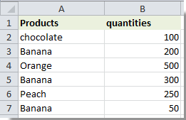
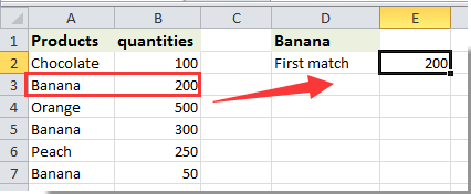
สมมติว่าคุณมีสองคอลัมน์ที่มีผลิตภัณฑ์และปริมาณดังภาพด้านล่างที่แสดง หากต้องการทราบปริมาณกล้วยลูกแรกหรือลูกที่สองอย่างรวดเร็วคุณจะทำอย่างไร?

ฟังก์ชั่น vlookup สามารถช่วยคุณจัดการกับปัญหานี้ได้ ในบทความนี้เราจะแสดงวิธี vlookup ค้นหาค่าการจับคู่แรกวินาทีหรือที่ n ด้วยฟังก์ชัน Vlookup ใน Excel

Vlookup ค้นหาค่าการจับคู่ครั้งแรกที่ 2 หรือที่ n ใน Excel ด้วยสูตร

vlookup ค้นหาค่าการจับคู่แรกใน Excel ได้อย่างง่ายดายด้วย Kutools for Excel


Vlookup ค้นหาค่าการจับคู่ครั้งแรก 2 หรือที่ n ใน Excel

โปรดทำดังนี้เพื่อค้นหาค่าการจับคู่ครั้งแรกที่ 2 หรือที่ n ใน Excel

1. ในเซลล์ D1 ป้อนเกณฑ์ที่คุณต้องการ vlookup ที่นี่ฉันป้อน Banana

2. ที่นี่เราจะพบมูลค่าการจับคู่แรกของกล้วย เลือกเซลล์ว่างเช่น E2 คัดลอกและวางสูตร =INDEX($B$2:$B$6,MATCH(TRUE,EXACT($D$1,$A$2:$A$6),0)) ลงในแถบสูตรแล้วกด Ctrl + เปลี่ยน + เข้าสู่ คีย์พร้อมกัน

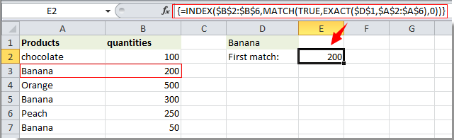
หมายเหตุ: ในสูตรนี้ $ B $ 2: $ B $ 6 คือช่วงของค่าที่ตรงกัน $ A $ 2: $ A $ 6 คือช่วงที่มีเกณฑ์ทั้งหมดสำหรับ vlookup $ D $ 1 คือเซลล์ที่มีเกณฑ์ vlookup ที่ระบุ

จากนั้นคุณจะได้รับค่าการจับคู่แรกของกล้วยในเซลล์ E2 ด้วยสูตรนี้คุณจะได้รับเฉพาะค่าแรกที่สอดคล้องกันตามเกณฑ์ของคุณ

หากต้องการรับค่าสัมพัทธ์ที่ n คุณสามารถใช้สูตรต่อไปนี้: =INDEX($B$2:$B$6,SMALL(IF($D$1=$A$2:$A$6,ROW($A$2:$A$6)-ROW($A$2)+1),1)) + Ctrl + เปลี่ยน + เข้าสู่ เข้าด้วยกันสูตรนี้จะส่งคืนค่าที่ตรงกันแรก

หมายเหตุ / รายละเอียดเพิ่มเติม:

1. หากต้องการค้นหาค่าการจับคู่ที่สองโปรดเปลี่ยนสูตรด้านบนเป็น =INDEX($B$2:$B$6,SMALL(IF($D$1=$A$2:$A$6,ROW($A$2:$A$6)-ROW($A$2)+1),2))จากนั้นกด Ctrl + เปลี่ยน + เข้าสู่ คีย์พร้อมกัน ดูภาพหน้าจอ:

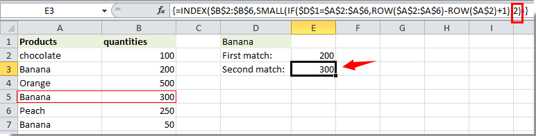
2. ตัวเลขสุดท้ายในสูตรข้างต้นหมายถึงค่าการจับคู่ที่ n ของเกณฑ์ vlookup หากคุณเปลี่ยนเป็น 3 จะได้ค่าการจับคู่ที่สามและเปลี่ยนเป็น n จะพบค่าการจับคู่ที่ n


Vlookup ค้นหาค่าการจับคู่แรกใน Excel ด้วย Kutools for Excel

Yคุณสามารถค้นหาค่าการจับคู่แรกใน Excel ได้อย่างง่ายดายโดยไม่ต้องจำสูตรด้วย มองหาค่าในรายการ สูตรสูตรของ Kutools สำหรับ Excel.

ก่อนที่จะใช้ Kutools สำหรับ Excelโปรด ดาวน์โหลดและติดตั้งในตอนแรก.

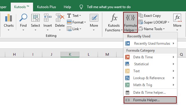
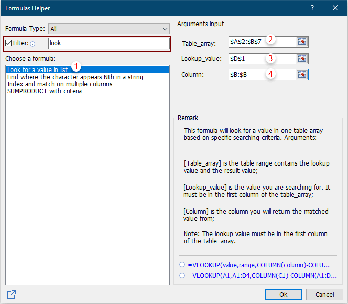
1. เลือกเซลล์สำหรับค้นหาค่าที่ตรงกันแรก (เซลล์ E2 กล่าวว่า) จากนั้นคลิก Kutools > ตัวช่วยสูตร > ตัวช่วยสูตร. ดูภาพหน้าจอ:

3 ใน ตัวช่วยสูตร โปรดกำหนดค่าดังต่อไปนี้:

  • 3.1 ใน เลือกสูตร ค้นหาและเลือก มองหาค่าในรายการ;
    เคล็ดลับ: คุณสามารถตรวจสอบไฟล์ ตัวกรอง ป้อนคำบางคำลงในกล่องข้อความเพื่อกรองสูตรอย่างรวดเร็ว
  • 3.2 ใน Table_array เลือกกล่อง ตารางซึ่งมีค่าค่าแรกที่ตรงกัน;
  • 3.2 ใน lookup_value ให้เลือกเซลล์ที่มีไฟล์ เกณฑ์ คุณจะส่งคืนค่าแรกตาม;
  • 3.3 ใน คอลัมน์ ระบุคอลัมน์ที่คุณจะส่งคืนค่าที่ตรงกันจาก หรือคุณสามารถป้อนหมายเลขคอลัมน์ลงในกล่องข้อความได้โดยตรงตามที่คุณต้องการ
  • 3.4 คลิกปุ่ม OK ปุ่ม. ดูภาพหน้าจอ:

ตอนนี้ค่าของเซลล์ที่เกี่ยวข้องจะถูกเติมอัตโนมัติในเซลล์ C10 ตามการเลือกรายการแบบเลื่อนลง

  หากคุณต้องการทดลองใช้ยูทิลิตีนี้ฟรี (30 วัน) กรุณาคลิกเพื่อดาวน์โหลดแล้วไปใช้การดำเนินการตามขั้นตอนข้างต้น

สุดยอดเครื่องมือเพิ่มผลผลิตในสำนักงาน

🤖 Kutools AI ผู้ช่วย: ปฏิวัติการวิเคราะห์ข้อมูลโดยยึดตาม: การดำเนินการที่ชาญฉลาด   |  สร้างรหัส  |  สร้างสูตรที่กำหนดเอง  |  วิเคราะห์ข้อมูลและสร้างแผนภูมิ  |  เรียกใช้ฟังก์ชัน Kutools...
คุณสมบัติยอดนิยม: ค้นหา เน้น หรือระบุรายการที่ซ้ำกัน   |  ลบแถวว่าง   |  รวมคอลัมน์หรือเซลล์โดยไม่สูญเสียข้อมูล   |   รอบโดยไม่มีสูตร ...
การค้นหาขั้นสูง: VLookup หลายเกณฑ์    VLookup หลายค่า  |   VLookup ข้ามหลายแผ่น   |   การค้นหาที่ไม่ชัดเจน ....
รายการแบบเลื่อนลงขั้นสูง: สร้างรายการแบบหล่นลงอย่างรวดเร็ว   |  รายการแบบหล่นลงขึ้นอยู่กับ   |  เลือกหลายรายการแบบหล่นลง ....
ผู้จัดการคอลัมน์: เพิ่มจำนวนคอลัมน์เฉพาะ  |  ย้ายคอลัมน์  |  สลับสถานะการมองเห็นของคอลัมน์ที่ซ่อนอยู่  |  เปรียบเทียบช่วงและคอลัมน์ ...
คุณสมบัติเด่น: กริดโฟกัส   |  มุมมองการออกแบบ   |   บาร์สูตรใหญ่    สมุดงานและตัวจัดการชีต   |  ห้องสมุดทรัพยากร (ข้อความอัตโนมัติ)   |  เลือกวันที่   |  รวมแผ่นงาน   |  เข้ารหัส/ถอดรหัสเซลล์    ส่งอีเมลตามรายการ   |  ซุปเปอร์ฟิลเตอร์   |   ตัวกรองพิเศษ (กรองตัวหนา/ตัวเอียง/ขีดทับ...) ...
ชุดเครื่องมือ 15 อันดับแรก12 ข้อความ เครื่องมือ (เพิ่มข้อความ, ลบอักขระ, ... )   |   50 + แผนภูมิ ประเภท (แผนภูมิ Gantt, ... )   |   40+ ใช้งานได้จริง สูตร (คำนวณอายุตามวันเกิด, ... )   |   19 การแทรก เครื่องมือ (ใส่ QR Code, แทรกรูปภาพจากเส้นทาง, ... )   |   12 การแปลง เครื่องมือ (ตัวเลขเป็นคำ, การแปลงสกุลเงิน, ... )   |   7 ผสานและแยก เครื่องมือ (แถวรวมขั้นสูง, แยกเซลล์, ... )   |   ... และอื่น ๆ

เพิ่มพูนทักษะ Excel ของคุณด้วย Kutools สำหรับ Excel และสัมผัสประสิทธิภาพอย่างที่ไม่เคยมีมาก่อน Kutools สำหรับ Excel เสนอคุณสมบัติขั้นสูงมากกว่า 300 รายการเพื่อเพิ่มประสิทธิภาพและประหยัดเวลา  คลิกที่นี่เพื่อรับคุณสมบัติที่คุณต้องการมากที่สุด...

รายละเอียด


แท็บ Office นำอินเทอร์เฟซแบบแท็บมาที่ Office และทำให้งานของคุณง่ายขึ้นมาก

  • เปิดใช้งานการแก้ไขและอ่านแบบแท็บใน Word, Excel, PowerPoint, ผู้จัดพิมพ์, Access, Visio และโครงการ
  • เปิดและสร้างเอกสารหลายรายการในแท็บใหม่ของหน้าต่างเดียวกันแทนที่จะเป็นในหน้าต่างใหม่
  • เพิ่มประสิทธิภาพการทำงานของคุณ 50% และลดการคลิกเมาส์หลายร้อยครั้งให้คุณทุกวัน!
Comments (43)
No ratings yet. Be the first to rate!
This comment was minimized by the moderator on the site
You only return first match with VLOOKUP so your article "How To Vlookup Find The First, 2nd Or Nth Match Value In Excel?" does not make any sense....
This comment was minimized by the moderator on the site
Hi Sima,
"VLOOKUP" is a Google search term, so I used it as a keyword for the article title. The main operation of this article is to lookup values. I'm sorry for the misunderstanding.
This comment was minimized by the moderator on the site
What if the next record on col b is a duplicate how do ignore duplicate? Let's Banana has quantities of 200 twice? Can you please help me figure out how to ignore the duplicate?
This comment was minimized by the moderator on the site
Cna anybody Explain the small function with the IF statement for me please? I don't really understand how that array works :(
This comment was minimized by the moderator on the site
The following formulas works perfect for me:
(a) or(b) =IF(H8='Raw Data'!B4,INDEX('Raw Data'!H6:H20,SMALL(IF(C18='Raw Data'!B6:B20,ROW('Raw Data'!B6:B20)-ROW('Raw Data'!B6:B20)+1),1)))

However, I have encountered a problem where there are 7 sets of the same criteria but in different columns:(1) can the above formula (a) be repeated and search in a different cells in a single formula and(2) the above formula (b) only allows up to two sets of the similar search with matched value result but when trying for the third set in the formula as showed below, Microsoft Excel appeared as "You've entered too many arguments for this function."
=<span style="letter-spacing: 0.2px; color: inherit; font-family: inherit; font-style: inherit; font-variant-ligatures: inherit; font-variant-caps: inherit; font-weight: inherit;">IF(H8='Raw Data'!J4,INDEX('Raw Data'!P6:P20,SMALL(IF(C18='Raw Data'!J6:J20,ROW('Raw Data'!J6:J20)-ROW('Raw Data'!J6:J20)+1),1))),</span>
This comment was minimized by the moderator on the site
What do Ctrl + Shift + Enter do?? At the beginning I didn'
This comment was minimized by the moderator on the site
Hi,An array formula needs to hit the Ctrl + Shift + Enter keys simultaneously to get the correct result.
This comment was minimized by the moderator on the site
I have a scenario... How do I get last price of anything for reference... Example: Banana first price was 200... While purchasing for second time; I need to display 200 in my expected price cell and then if I buy that on the day at 220, I will put this value manually as 220... Whenever next time I will buy banana; I need to display 220 from the last purchase price
This comment was minimized by the moderator on the site
Try =INDEX($B$2:$B$6,XMATCH(TRUE,EXACT($D$1,$A$2:$A$6),0,-1))

This is essentially reversing the search order and returning the first match using the XMATCH function.

Better late than never, hopefully helps someone :)
This comment was minimized by the moderator on the site
Perfect explanation, thanks.
This comment was minimized by the moderator on the site
If the first or any of the other entry's for 'banana' column B was blank cell, of which I don't require this number, what changes are required to this formula to skip blank cell in column B.
This comment was minimized by the moderator on the site
Sorry I am using this formula
=INDEX($B$2:$B$6,SMALL(IF($D$1=$A$2:$A$6,ROW($A$2:$A$6)-ROW($A$2)+1),1))
This comment was minimized by the moderator on the site
SOLVED:
=SMALL(IF(A2:A7=D1,IF(B2:B7<>"",B2:B7)),1)

If 2nd or 3rd number required exchange ),1) to 2 or 3

This formula does not require index, as it directly looks at the value in Cell
This comment was minimized by the moderator on the site
Correction to previous formula:
The value was reading either the lesser or greater.

Updated formula
=INDEX($B$2:$B$7,SMALL(IF($A2:$A6=$D$1,IF($B$2:$B$7<>"",ROW($A2:$A6)-ROW($A2)+1)),1))

This skips blank cell and places value of non blank cell. Replace +1 with +2 or +3 for 2nd or 3rd value
This comment was minimized by the moderator on the site
And if you want the last, second last, nth last just add a counter (count the number of events already hapenned) to the end and subtract it by 0,1,n respectively.

Thank you so much! I was searching for this for a long time
This comment was minimized by the moderator on the site
Good Day,
Sorry can't help you with this yet. Thank you for your comment.
This comment was minimized by the moderator on the site
Is it possible to find an average of the non-unique data. Or would it be possible to have a list dropdown on the cell of the various values?
This comment was minimized by the moderator on the site
Good Day,
Sorry can't help you with this yet. Thank you for your comment.
There are no comments posted here yet
Load More
Please leave your comments in English
Posting as Guest
×
Rate this post:
0   Characters
Suggested Locations